18. The Aiyagari Model#
GPU
This lecture was built using a machine with access to a GPU — although it will also run without one.
Google Colab has a free tier with GPUs that you can access as follows:
Click on the “play” icon top right
Select Colab
Set the runtime environment to include a GPU
18.1. Overview#
In this lecture, we describe the structure of a class of models that build on work by Truman Bewley [Bew77].
We begin by discussing an example of a Bewley model due to Rao Aiyagari [Aiy94].
The model features
Heterogeneous agents
A single exogenous vehicle for borrowing and lending
Limits on amounts individual agents may borrow
The Aiyagari model has been used to investigate many topics, including
precautionary savings and the effect of liquidity constraints [Aiy94]
risk sharing and asset pricing [HL96]
the shape of the wealth distribution [BBZ15]
18.1.1. References#
The primary reference for this lecture is [Aiy94].
A textbook treatment is available in chapter 18 of [LS18].
A less sophisticated version of this lecture (without JAX) can be found here.
18.1.2. Preliminaries#
We use the following imports
import time
import matplotlib.pyplot as plt
import numpy as np
import jax
import jax.numpy as jnp
from collections import namedtuple
Let’s check the GPU we are running
!nvidia-smi
Fri Jun 26 06:36:54 2026
+-----------------------------------------------------------------------------------------+
| NVIDIA-SMI 580.105.08             Driver Version: 580.105.08     CUDA Version: 13.0     |
+-----------------------------------------+------------------------+----------------------+
| GPU  Name                 Persistence-M | Bus-Id          Disp.A | Volatile Uncorr. ECC |
| Fan  Temp   Perf          Pwr:Usage/Cap |           Memory-Usage | GPU-Util  Compute M. |
|                                         |                        |               MIG M. |
|=========================================+========================+======================|
|   0  Tesla T4                       On  |   00000000:00:1E.0 Off |                    0 |
| N/A   26C    P8              9W /   70W |       0MiB /  15360MiB |      0%      Default |
|                                         |                        |                  N/A |
+-----------------------------------------+------------------------+----------------------+

+-----------------------------------------------------------------------------------------+
| Processes:                                                                              |
|  GPU   GI   CI              PID   Type   Process name                        GPU Memory |
|        ID   ID                                                               Usage      |
|=========================================================================================|
|  No running processes found                                                             |
+-----------------------------------------------------------------------------------------+
We will use 64 bit floats with JAX in order to increase the precision.
jax.config.update("jax_enable_x64", True)
We will use the following function to compute stationary distributions of stochastic matrices. (For a reference to the algorithm, see p. 88 of Economic Dynamics.)
@jax.jit
def compute_stationary(P):
    n = P.shape[0]
    I = jnp.identity(n)
    O = jnp.ones((n, n))
    A = I - jnp.transpose(P) + O
    return jnp.linalg.solve(A, jnp.ones(n))
18.2. Firms#
Firms produce output by hiring capital and labor.
Firms act competitively and face constant returns to scale.
Since returns to scale are constant the number of firms does not matter.
Hence we can consider a single (but nonetheless competitive) representative firm.
The firm’s output is
where
\( A \) and \( \alpha \) are parameters with \( A > 0 \) and \( \alpha \in (0, 1) \)
\( K\) is aggregate capital
\( N \) is total labor supply (which is constant in this simple version of the model)
The firm’s problem is
The parameter \( \delta \) is the depreciation rate.
These parameters are stored in the following namedtuple.
Firm = namedtuple('Firm', ('A', 'N', 'α', 'δ'))

def create_firm(A=1.0,
                N=1.0,
                α=0.33,
                δ=0.05):
    """
    Create a namedtuple that stores firm data.

    """
    return Firm(A=A, N=N, α=α, δ=δ)
From the first-order condition with respect to capital, the firm’s inverse demand for capital is
def r_given_k(K, firm):
    """
    Inverse demand curve for capital.  The interest rate associated with a
    given demand for capital K.
    """
    A, N, α, δ = firm
    return A * α * (N / K)**(1 - α) - δ
Using (18.1) and the firm’s first-order condition for labor,
def r_to_w(r, firm):
    """
    Equilibrium wages associated with a given interest rate r.
    """
    A, N, α, δ = firm
    return A * (1 - α) * (A * α / (r + δ))**(α / (1 - α))
18.3. Households#
Infinitely lived households / consumers face idiosyncratic income shocks.
A unit interval of ex-ante identical households face a common borrowing constraint.
The savings problem faced by a typical household is
subject to
where
\( c_t \) is current consumption
\( a_t \) is assets
\( z_t \) is an exogenous component of labor income capturing stochastic unemployment risk, etc.
\( w \) is a wage rate
\( r \) is a net interest rate
\( B \) is the maximum amount that the agent is allowed to borrow
The exogenous process \( \{z_t\} \) follows a finite state Markov chain with given stochastic matrix \( P \).
In this simple version of the model, households supply labor inelastically because they do not value leisure.
Below we provide code to solve the household problem, taking \(r\) and \(w\) as fixed.
18.3.1. Primitives and Operators#
We will solve the household problem using Howard policy iteration (see Ch 5 of Dynamic Programming).
First we set up a namedtuple to store the parameters that define a household asset accumulation problem, as well as the grids used to solve it.
Household = namedtuple('Household',
                       ('β', 'a_grid', 'z_grid', 'Π'))
def create_household(β=0.96,                      # Discount factor
                     Π=[[0.9, 0.1], [0.1, 0.9]],  # Markov chain
                     z_grid=[0.1, 1.0],           # Exogenous states
                     a_min=1e-10, a_max=20,       # Asset grid
                     a_size=200):
    """
    Create a namedtuple that stores all data needed to solve the household
    problem, given prices.

    """
    a_grid = jnp.linspace(a_min, a_max, a_size)
    z_grid, Π = map(jnp.array, (z_grid, Π))
    return Household(β=β, a_grid=a_grid, z_grid=z_grid, Π=Π)
For now we assume that \(u(c) = \log(c)\).
(CRRA utility is treated in the exercises.)
u = jnp.log
Here’s a tuple that stores the wage rate and interest rate, as well as a function that creates a price namedtuple with default values.
Prices = namedtuple('Prices', ('r', 'w'))

def create_prices(r=0.01,   # Interest rate
                  w=1.0):   # Wages
    return Prices(r=r, w=w)
Now we set up a vectorized version of the right-hand side of the Bellman equation (before maximization), which is a 3D array representing
for all \((a, z, a')\).
@jax.jit
def B(v, household, prices):
    # Unpack
    β, a_grid, z_grid, Π = household
    a_size, z_size = len(a_grid), len(z_grid)
    r, w = prices

    # Compute current consumption as array c[i, j, ip]
    a  = jnp.reshape(a_grid, (a_size, 1, 1))    # a[i]   ->  a[i, j, ip]
    z  = jnp.reshape(z_grid, (1, z_size, 1))    # z[j]   ->  z[i, j, ip]
    ap = jnp.reshape(a_grid, (1, 1, a_size))    # ap[ip] -> ap[i, j, ip]
    c = w * z + (1 + r) * a - ap

    # Calculate continuation rewards at all combinations of (a, z, ap)
    v = jnp.reshape(v, (1, 1, a_size, z_size))  # v[ip, jp] -> v[i, j, ip, jp]
    Π = jnp.reshape(Π, (1, z_size, 1, z_size))  # Π[j, jp]  -> Π[i, j, ip, jp]
    EV = jnp.sum(v * Π, axis=-1)                 # sum over last index jp

    # Compute the right-hand side of the Bellman equation
    return jnp.where(c > 0, u(c) + β * EV, -jnp.inf)
The next function computes greedy policies.
@jax.jit
def get_greedy(v, household, prices):
    """
    Computes a v-greedy policy σ, returned as a set of indices.  If
    σ[i, j] equals ip, then a_grid[ip] is the maximizer at i, j.

    """
    return jnp.argmax(B(v, household, prices), axis=-1) # argmax over ap
The following function computes the array \(r_{\sigma}\) which gives current rewards given policy \(\sigma\).
@jax.jit
def compute_r_σ(σ, household, prices):
    """
    Compute current rewards at each i, j under policy σ.  In particular,

        r_σ[i, j] = u((1 + r)a[i] + wz[j] - a'[ip])

    when ip = σ[i, j].

    """
    # Unpack
    β, a_grid, z_grid, Π = household
    a_size, z_size = len(a_grid), len(z_grid)
    r, w = prices

    # Compute r_σ[i, j]
    a = jnp.reshape(a_grid, (a_size, 1))
    z = jnp.reshape(z_grid, (1, z_size))
    ap = a_grid[σ]
    c = (1 + r) * a + w * z - ap
    r_σ = u(c)

    return r_σ
The value \(v_{\sigma}\) of a policy \(\sigma\) is defined as
(See Ch 5 of Dynamic Programming for notation and background on Howard policy iteration.)
To compute this vector, we set up the linear map \(v \rightarrow R_{\sigma} v\), where \(R_{\sigma} := I - \beta P_{\sigma}\).
This map can be expressed as
(Notice that \(R_\sigma\) is expressed as a linear operator rather than a matrix – this is much easier and cleaner to code, and also exploits sparsity.)
@jax.jit
def R_σ(v, σ, household):
    # Unpack
    β, a_grid, z_grid, Π = household
    a_size, z_size = len(a_grid), len(z_grid)

    # Set up the array v[σ[i, j], jp]
    zp_idx = jnp.arange(z_size)
    zp_idx = jnp.reshape(zp_idx, (1, 1, z_size))
    σ = jnp.reshape(σ, (a_size, z_size, 1))
    V = v[σ, zp_idx]

    # Expand Π[j, jp] to Π[i, j, jp]
    Π = jnp.reshape(Π, (1, z_size, z_size))

    # Compute and return v[i, j] - β Σ_jp v[σ[i, j], jp] * Π[j, jp]
    return v - β * jnp.sum(V * Π, axis=-1)
The next function computes the lifetime value of a given policy.
@jax.jit
def get_value(σ, household, prices):
    """
    Get the lifetime value of policy σ by computing

        v_σ = R_σ^{-1} r_σ

    """
    r_σ = compute_r_σ(σ, household, prices)
    # Reduce R_σ to a function in v
    _R_σ = lambda v: R_σ(v, σ, household)
    # Compute v_σ = R_σ^{-1} r_σ using an iterative routing.
    return jax.scipy.sparse.linalg.bicgstab(_R_σ, r_σ)[0]
Here’s the Howard policy iteration.
def howard_policy_iteration(household, prices,
                            tol=1e-4, max_iter=10_000, verbose=False):
    """
    Howard policy iteration routine.

    """
    β, a_grid, z_grid, Π = household
    a_size, z_size = len(a_grid), len(z_grid)
    σ = jnp.zeros((a_size, z_size), dtype=int)

    v_σ = get_value(σ, household, prices)
    i = 0
    error = tol + 1
    while error > tol and i < max_iter:
        σ_new = get_greedy(v_σ, household, prices)
        v_σ_new = get_value(σ_new, household, prices)
        error = jnp.max(jnp.abs(v_σ_new - v_σ))
        σ = σ_new
        v_σ = v_σ_new
        i = i + 1
        if verbose:
            print(f"Concluded loop {i} with error {error}.")
    return σ
As a first example of what we can do, let’s compute and plot an optimal accumulation policy at fixed prices.
# Create an instance of Household
household = create_household()
prices = create_prices()
r, w = prices
r, w
(0.01, 1.0)
%time σ_star = howard_policy_iteration(household, prices, verbose=True)
Concluded loop 1 with error 11.366831579022996.
Concluded loop 2 with error 9.574522771860245.
Concluded loop 3 with error 3.9654760004604777.
Concluded loop 4 with error 1.1207075306313232.
Concluded loop 5 with error 0.2524013153055833.
Concluded loop 6 with error 0.12172293662906064.
Concluded loop 7 with error 0.043395682867316765.
Concluded loop 8 with error 0.012132319676439351.
Concluded loop 9 with error 0.005822155404443308.
Concluded loop 10 with error 0.002863165320343697.
Concluded loop 11 with error 0.0016657175376657563.
Concluded loop 12 with error 0.0004143776102245589.
Concluded loop 13 with error 0.0.
CPU times: user 846 ms, sys: 44.6 ms, total: 890 ms
Wall time: 751 ms
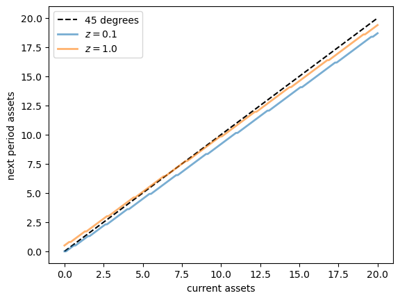
The next plot shows asset accumulation policies at different values of the exogenous state.
β, a_grid, z_grid, Π = household

fig, ax = plt.subplots()
ax.plot(a_grid, a_grid, 'k--', label="45 degrees")
for j, z in enumerate(z_grid):
    lb = f'$z = {z:.2}$'
    policy_vals = a_grid[σ_star[:, j]]
    ax.plot(a_grid, policy_vals, lw=2, alpha=0.6, label=lb)
    ax.set_xlabel('current assets')
    ax.set_ylabel('next period assets')
ax.legend(loc='upper left')
plt.show()
18.3.2. Capital Supply#
To start thinking about equilibrium, we need to know how much capital households supply at a given interest rate \(r\).
This quantity can be calculated by taking the stationary distribution of assets under the optimal policy and computing the mean.
The next function computes the stationary distribution for a given policy \(\sigma\) via the following steps:
compute the stationary distribution \(\psi = (\psi(a, z))\) of \(P_{\sigma}\), which defines the Markov chain of the state \((a_t, z_t)\) under policy \(\sigma\).
sum out \(z_t\) to get the marginal distribution for \(a_t\).
@jax.jit
def compute_asset_stationary(σ, household):
    # Unpack
    β, a_grid, z_grid, Π = household
    a_size, z_size = len(a_grid), len(z_grid)

    # Construct P_σ as an array of the form P_σ[i, j, ip, jp]
    ap_idx = jnp.arange(a_size)
    ap_idx = jnp.reshape(ap_idx, (1, 1, a_size, 1))
    σ = jnp.reshape(σ, (a_size, z_size, 1, 1))
    A = jnp.where(σ == ap_idx, 1, 0)
    Π = jnp.reshape(Π, (1, z_size, 1, z_size))
    P_σ = A * Π

    # Reshape P_σ into a matrix
    n = a_size * z_size
    P_σ = jnp.reshape(P_σ, (n, n))

    # Get stationary distribution and reshape back onto [i, j] grid
    ψ = compute_stationary(P_σ)
    ψ = jnp.reshape(ψ, (a_size, z_size))

    # Sum along the rows to get the marginal distribution of assets
    ψ_a = jnp.sum(ψ, axis=1)
    return ψ_a
Let’s give this a test run.
ψ_a = compute_asset_stationary(σ_star, household)
fig, ax = plt.subplots()
ax.bar(household.a_grid, ψ_a)
ax.set_xlabel("asset level")
ax.set_ylabel("probability mass")
plt.show()
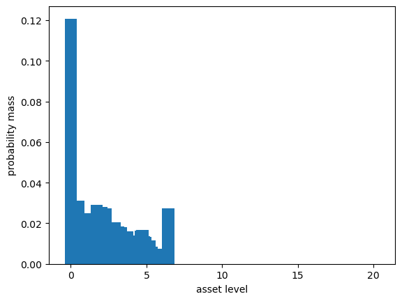
The distribution should sum to one:
ψ_a.sum()
Array(1., dtype=float64)
The next function computes aggregate capital supply by households under policy \(\sigma\), given wages and interest rates.
def capital_supply(σ, household):
    """
    Induced level of capital stock under the policy, taking r and w as given.

    """
    β, a_grid, z_grid, Π = household
    ψ_a = compute_asset_stationary(σ, household)
    return float(jnp.sum(ψ_a * a_grid))
18.4. Equilibrium#
We compute a stationary rational expectations equilibrium (SREE) as follows:
set \(n=0\), start with initial guess \( K_0\) for aggregate capital
determine prices \(r, w\) from the firm decision problem, given \(K_n\)
compute the optimal savings policy of the households given these prices
compute aggregate capital \(K_{n+1}\) as the mean of steady state capital given this savings policy
if \(K_{n+1} \approx K_n\) stop, otherwise go to step 2.
We can write the sequence of operations in steps 2-4 as
If \(K_{n+1}\) agrees with \(K_n\) then we have a SREE.
In other words, our problem is to find the fixed-point of the one-dimensional map \(G\).
Here’s \(G\) expressed as a Python function:
def G(K, firm, household):
    # Get prices r, w associated with K
    r = r_given_k(K, firm)
    w = r_to_w(r, firm)
    # Generate a household object with these prices, compute
    # aggregate capital.
    prices = create_prices(r=r, w=w)
    σ_star = howard_policy_iteration(household, prices)
    return capital_supply(σ_star, household)
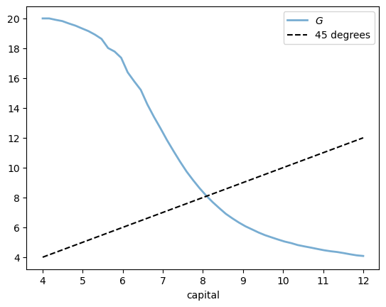
18.4.1. Visual inspection#
Let’s inspect visually as a first pass.
num_points = 50
firm = create_firm()
household = create_household()
k_vals = np.linspace(4, 12, num_points)
out = [G(k, firm, household) for k in k_vals]
fig, ax = plt.subplots()
ax.plot(k_vals, out, lw=2, alpha=0.6, label='$G$')
ax.plot(k_vals, k_vals, 'k--', label="45 degrees")
ax.set_xlabel('capital')
ax.legend()
plt.show()
18.4.2. Computing the equilibrium#
Now let’s compute the equilibrium.
Looking at the figure above, we see that a simple iteration scheme \(K_{n+1} = G(K_n)\) will cycle from high to low values, leading to slow convergence.
As a result, we use a damped iteration scheme of the form
def compute_equilibrium(firm, household,
                        K0=6, α=0.99, max_iter=1_000, tol=1e-4,
                        print_skip=10, verbose=False):
    n = 0
    K = K0
    error = tol + 1
    while error > tol and n < max_iter:
        new_K = α * K + (1 - α) * G(K, firm, household)
        error = abs(new_K - K)
        K = new_K
        n += 1
        if verbose and n % print_skip == 0:
            print(f"At iteration {n} with error {error}")
    return K, n
firm = create_firm()
household = create_household()
print("\nComputing equilibrium capital stock")
start = time.time()
K_star, n = compute_equilibrium(firm, household, K0=6.0, verbose=True)
elapsed = time.time() - start
print(f"Computed equilibrium {K_star:.5} in {n} iterations and {elapsed} seconds")
Computing equilibrium capital stock
At iteration 10 with error 0.06490545798825043
At iteration 20 with error 0.03626685465742874
At iteration 30 with error 0.021452703682580676
At iteration 40 with error 0.013383829253038826
At iteration 50 with error 0.008397515264451982
At iteration 60 with error 0.005656370053102933
At iteration 70 with error 0.003750107819944226
At iteration 80 with error 0.0024816210955460605
At iteration 90 with error 0.0017352118525710836
At iteration 100 with error 0.0009559876839571047
At iteration 110 with error 0.0006843412658508186
At iteration 120 with error 0.00046762845631675987
At iteration 130 with error 0.00038193101011607666
At iteration 140 with error 0.00019421626809901227
At iteration 150 with error 0.00017041810881579522
At iteration 160 with error 0.00015412308287032772
At iteration 170 with error 0.00013938615349395889
Computed equilibrium 8.0918 in 176 iterations and 39.43909811973572 seconds
This is not very fast, given how quickly we can solve the household problem.
You can try varying \(\alpha\), but usually this parameter is hard to set a priori.
In the exercises below you will be asked to use bisection instead, which generally performs better.
18.5. Exercises#
Exercise 18.1
Write a new version of compute_equilibrium that uses bisect from scipy.optimize instead of damped iteration.
See if you can make it faster that the previous version.
In bisect,
you should set
xtol=1e-4to have the same error tolerance as the previous version.for the lower and upper bounds of the bisection routine try
a = 1.0andb = 20.0.
Solution
from scipy.optimize import bisect
We use bisection to find the zero of the function \(h(k) = k - G(k)\).
def compute_equilibrium(firm, household, a=1.0, b=20.0):
    K = bisect(lambda k: k - G(k, firm, household), a, b, xtol=1e-4)
    return K
firm = create_firm()
household = create_household()
print("\nComputing equilibrium capital stock")
start = time.time()
K_star = compute_equilibrium(firm, household)
elapsed = time.time() - start
print(f"Computed equilibrium capital stock {K_star:.5} in {elapsed} seconds")
Computing equilibrium capital stock
Computed equilibrium capital stock 8.0938 in 0.923210620880127 seconds
Bisection seems to be faster than the damped iteration scheme.
Exercise 18.2
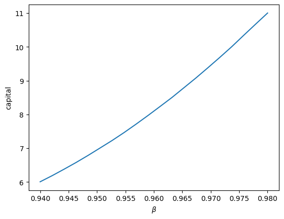
Show how equilibrium capital stock changes with \(\beta\).
Use the following values of \(\beta\) and plot the relationship you find.
β_vals = np.linspace(0.94, 0.98, 20)
Solution
K_vals = np.empty_like(β_vals)
K = 6.0  # initial guess

for i, β in enumerate(β_vals):
    household = create_household(β=β)
    K = compute_equilibrium(firm, household, 0.5 * K, 1.5 * K)
    print(f"Computed equilibrium {K:.4} at β = {β}")
    K_vals[i] = K
Computed equilibrium 6.006 at β = 0.94
Computed equilibrium 6.186 at β = 0.9421052631578947
Computed equilibrium 6.379 at β = 0.9442105263157894
Computed equilibrium 6.577 at β = 0.9463157894736841
Computed equilibrium 6.786 at β = 0.9484210526315789
Computed equilibrium 7.005 at β = 0.9505263157894737
Computed equilibrium 7.226 at β = 0.9526315789473684
Computed equilibrium 7.461 at β = 0.9547368421052631
Computed equilibrium 7.709 at β = 0.9568421052631578
Computed equilibrium 7.966 at β = 0.9589473684210525
Computed equilibrium 8.231 at β = 0.9610526315789474
Computed equilibrium 8.499 at β = 0.9631578947368421
Computed equilibrium 8.787 at β = 0.9652631578947368
Computed equilibrium 9.076 at β = 0.9673684210526315
Computed equilibrium 9.378 at β = 0.9694736842105263
Computed equilibrium 9.687 at β = 0.971578947368421
Computed equilibrium 10.0 at β = 0.9736842105263157
Computed equilibrium 10.34 at β = 0.9757894736842105
Computed equilibrium 10.67 at β = 0.9778947368421053
Computed equilibrium 11.0 at β = 0.98
fig, ax = plt.subplots()
ax.plot(β_vals, K_vals, ms=2)
ax.set_xlabel(r'$\beta$')
ax.set_ylabel('capital')
plt.show()