15. Inventory Management Model#

GPU

This lecture was built using a machine with access to a GPU.

Google Colab has a free tier with GPUs that you can access as follows:

Click on the “play” icon top right
Select Colab
Set the runtime environment to include a GPU

This lecture provides a JAX implementation of a model in Dynamic Programming.

In addition to JAX and Anaconda, this lecture will need the following libraries:

!pip install --upgrade quantecon

15.1. A model with constant discounting#

We study a firm where a manager tries to maximize shareholder value.

To simplify the problem, we assume that the firm only sells one product.

Letting \(\pi_t\) be profits at time \(t\) and \(r > 0\) be the interest rate, the value of the firm is

\[ V_0 = \sum_{t \geq 0} \beta^t \pi_t \qquad \text{ where } \quad \beta := \frac{1}{1+r}. \]

Suppose the firm faces exogenous demand process \((D_t)_{t \geq 0}\).

We assume \((D_t)_{t \geq 0}\) is IID with common distribution \(\phi \in (Z_+)\).

Inventory \((X_t)_{t \geq 0}\) of the product obeys

\[ X_{t+1} = f(X_t, D_{t+1}, A_t) \qquad \text{where} \quad f(x,a,d) := (x - d)\vee 0 + a. \]

The term \(A_t\) is units of stock ordered this period, which take one period to arrive.

We assume that the firm can store at most \(K\) items at one time.

Profits are given by

\[ \pi_t := X_t \wedge D_{t+1} - c A_t - \kappa 1\{A_t > 0\}. \]

We take the minimum of current stock and demand because orders in excess of inventory are assumed to be lost rather than back-filled.

Here \(c\) is unit product cost and \(\kappa\) is a fixed cost of ordering inventory.

We can map our inventory problem into a dynamic program with state space \(X := \{0, \ldots, K\}\) and action space \(A := X\).

The feasible correspondence \(\Gamma\) is

\[ \Gamma(x) := \{0, \ldots, K - x\}, \]

which represents the set of feasible orders when the current inventory state is \(x\).

The reward function is expected current profits, or

\[ r(x, a) := \sum_{d \geq 0} (x \wedge d) \phi(d) - c a - \kappa 1\{a > 0\}. \]

The stochastic kernel (i.e., state-transition probabilities) from the set of feasible state-action pairs is

\[ P(x, a, x') := P\{ f(x, a, D) = x' \} \qquad \text{when} \quad D \sim \phi. \]

When discounting is constant, the Bellman equation takes the form

(15.1)#\[ v(x) = \max_{a \in \Gamma(x)} \left\{ r(x, a) + \beta \sum_{d \geq 0} v(f(x, a, d)) \phi(d) \right\}\]

15.2. Time varing discount rates#

We wish to consider a more sophisticated model with time-varying discounting.

This time variation accommodates non-constant interest rates.

To this end, we replace the constant \(\beta\) in (15.1) with a stochastic process \((\beta_t)\) where

\(\beta_t = 1/(1+r_t)\) and
\(r_t\) is the interest rate at time \(t\)

We suppose that the dynamics can be expressed as \(\beta_t = \beta(Z_t)\), where the exogenous process \((Z_t)_{t \geq 0}\) is a Markov chain on \(Z\) with Markov matrix \(Q\).

After relabeling inventory \(X_t\) as \(Y_t\) and \(x\) as \(y\), the Bellman equation becomes

\[ v(y, z) = \max_{a \in \Gamma(x)} B((y, z), a, v) \]

where

(15.2)#\[ B((y, z), a, v) = r(y, a) + \beta(z) \sum_{d, \, z'} v(f(y, a, d), z') \phi(d) Q(z, z').\]

We set \(\beta(z) := z\) and

\[ R(y, a, y') := P\{f(y, a, d) = y'\} \quad \text{when} \quad D \sim \phi, \]

Now \(R(y, a, y')\) is the probability of realizing next period inventory level \(y'\) when the current level is \(y\) and the action is \(a\).

Hence we can rewrite (15.2) as

\[ B((y, z), a, v) = r(y, a) + \beta(z) \sum_{y', z'} v(y', z') Q(z, z') R(y, a, y') . \]

Let’s begin with the following imports

import quantecon as qe
import jax
import jax.numpy as jnp
import numpy as np
import matplotlib.pyplot as plt
from time import time
from functools import partial
from typing import NamedTuple

Let’s check the GPU we are running

!nvidia-smi

Mon Dec  8 03:42:28 2025       
+-----------------------------------------------------------------------------------------+
| NVIDIA-SMI 580.105.08             Driver Version: 580.105.08     CUDA Version: 13.0     |
+-----------------------------------------+------------------------+----------------------+
| GPU  Name                 Persistence-M | Bus-Id          Disp.A | Volatile Uncorr. ECC |
| Fan  Temp   Perf          Pwr:Usage/Cap |           Memory-Usage | GPU-Util  Compute M. |
|                                         |                        |               MIG M. |
|=========================================+========================+======================|
|   0  Tesla T4                       On  |   00000000:00:1E.0 Off |                    0 |
| N/A   29C    P8             13W /   70W |       0MiB /  15360MiB |      0%      Default |
|                                         |                        |                  N/A |
+-----------------------------------------+------------------------+----------------------+

+-----------------------------------------------------------------------------------------+
| Processes:                                                                              |
|  GPU   GI   CI              PID   Type   Process name                        GPU Memory |
|        ID   ID                                                               Usage      |
|=========================================================================================|
|  No running processes found                                                             |
+-----------------------------------------------------------------------------------------+

We will use 64 bit floats with JAX in order to increase the precision.

jax.config.update("jax_enable_x64", True)

Let’s define a model to represent the inventory management.

# NamedTuple Model
class Model(NamedTuple):
    z_values: jnp.ndarray        # Exogenous shock values
    Q: jnp.ndarray               # Exogenous shock probabilities
    x_values: jnp.ndarray        # Inventory values
    d_values: jnp.ndarray        # Demand values for summation
    ϕ_values: jnp.ndarray        # Demand probabilities
    p: float                     # Demand parameter
    c: float = 0.2               # Unit cost
    κ: float = 0.8               # Fixed cost

def create_sdd_inventory_model(
        ρ: float = 0.98,     # Exogenous state autocorrelation parameter
        ν: float = 0.002,    # Exogenous state volatility parameter
        n_z: int = 10,       # Exogenous state discretization size
        b: float = 0.97,     # Exogenous state offset
        K: int = 100,        # Max inventory
        D_MAX: int = 101,    # Demand upper bound for summation
        p: float = 0.6       
    ) -> Model:
    
    # Demand
    def demand_pdf(p, d):
        return (1 - p)**d * p
        
    d_values = jnp.arange(D_MAX)
    ϕ_values = demand_pdf(p, d_values)
    
    # Exogenous state process
    mc = qe.tauchen(n_z, ρ, ν)
    z_values, Q = map(jnp.array, (mc.state_values + b, mc.P))
    
    # Endogenous state
    x_values = jnp.arange(K + 1)   # 0, 1, ..., K
    
    return Model(
        z_values=z_values, Q=Q, 
        x_values=x_values, d_values=d_values, ϕ_values=ϕ_values,
        p=p
    )

Here’s the function B on the right-hand side of the Bellman equation.

@jax.jit
def B(x, z_idx, v, model):
    """
    Take z_idx and convert it to z.  Then compute

        B(x, z, a, v) = r(x, a) + β(z) Σ_x′ v(x′) P(x, a, x′)

    for all possible choices of a.
    """
    
    z_values, Q, x_values, d_values, ϕ_values, p, c, κ = model
    z = z_values[z_idx]

    def _B(a):
        """
        Returns r(x, a) + β(z) Σ_x′ v(x′) P(x, a, x′) for each a.
        """
        revenue = jnp.sum(jnp.minimum(x, d_values) * ϕ_values)
        profit = revenue - c * a - κ * (a > 0)
        v_R = jnp.sum(v[jnp.maximum(x - d_values, 0) + a].T * ϕ_values, axis=1)
        cv = jnp.sum(v_R * Q[z_idx])
        return profit + z * cv

    a_values = x_values   # Set of possible order sizes
    B_values = jax.vmap(_B)(a_values)
    max_x = len(x_values) - 1
    
    return jnp.where(a_values <= max_x - x, B_values, -jnp.inf)

We need to vectorize this function so that we can use it efficiently in JAX.

We apply a sequence of vmap operations to vectorize appropriately in each argument.

B = jax.vmap(B, in_axes=(None, 0, None, None))
B = jax.vmap(B, in_axes=(0, None, None, None))

Next we define the Bellman operator.

@jax.jit
def T(v, model):
    """The Bellman operator."""
    z_values, Q, x_values, d_values, ϕ_values, p, c, κ = model
    z_indices = jnp.arange(len(z_values))
    res = B(x_values, z_indices, v, model)
    return jnp.max(res, axis=2)

The following function computes a v-greedy policy.

@jax.jit
def get_greedy(v, model):
    """Get a v-greedy policy.  Returns a zero-based array."""
    z_values, Q, x_values, d_values, ϕ_values, p, c, κ = model
    z_indices = jnp.arange(len(z_values))
    res = B(x_values, z_indices, v, model)
    return jnp.argmax(res, axis=2)

Here’s code to solve the model using value function iteration.

@jax.jit
def solve_inventory_model(v_init, model, max_iter=10_000, tol=1e-6):
    """Use successive_approx to get v_star and then compute greedy."""

    def update(state):
        error, i, v = state
        new_v = T(v, model)
        new_error = jnp.max(jnp.abs(new_v - v))
        new_i = i + 1
        return new_error, new_i, new_v

    def test(state):
        error, i, v = state
        return (i < max_iter) & (error > tol)

    i, error = 0, tol + 1
    initial_state = error, i, v_init
    final_state = jax.lax.while_loop(test, update, initial_state)
    error, i, v_star = final_state
    σ_star = get_greedy(v_star, model)
    return v_star, σ_star

Now let’s create an instance and solve it.

model = create_sdd_inventory_model()
z_values, Q, x_values, d_values, ϕ_values, p, c, κ = model
n_z = len(z_values)
n_x = len(x_values)
v_init = jnp.zeros((n_x, n_z), dtype=float)

W1208 03:42:29.648024    3480 cuda_executor.cc:1802] GPU interconnect information not available: INTERNAL: NVML doesn't support extracting fabric info or NVLink is not used by the device.
W1208 03:42:29.651649    3414 cuda_executor.cc:1802] GPU interconnect information not available: INTERNAL: NVML doesn't support extracting fabric info or NVLink is not used by the device.

start = time()
v_star, σ_star = solve_inventory_model(v_init, model)

# Pause until execution finishes
jax.tree_util.tree_map(lambda x: x.block_until_ready(), (v_star, σ_star))

jax_time_with_compile = time() - start
print(f"compile plus execution time = {jax_time_with_compile * 1000:.6f} ms")

compile plus execution time = 1792.853355 ms

Let’s run again to get rid of the compile time.

start = time()
v_star, σ_star = solve_inventory_model(v_init, model)

# Pause until execution finishes
jax.tree_util.tree_map(lambda x: x.block_until_ready(), (v_star, σ_star))

jax_time_without_compile = time() - start
print(f"execution time = {jax_time_without_compile * 1000:.6f} ms")

execution time = 809.458494 ms

Now let’s do a simulation.

We’ll begin by converting back to NumPy arrays for convenience

Q = np.array(Q)
z_values = np.array(z_values)
z_mc = qe.MarkovChain(Q, z_values)

Here’s code to simulate inventories

def sim_inventories(ts_length, X_init=0):
    """Simulate given the optimal policy."""
    global p, z_mc
    
    z_idx = z_mc.simulate_indices(ts_length, init=1)
    X = np.zeros(ts_length, dtype=np.int32)
    X[0] = X_init
    rand = np.random.default_rng().geometric(p=p, size=ts_length-1) - 1
    
    for t in range(ts_length-1):
        X[t+1] = np.maximum(X[t] - rand[t], 0) + σ_star[X[t], z_idx[t]]
        
    return X, z_values[z_idx]

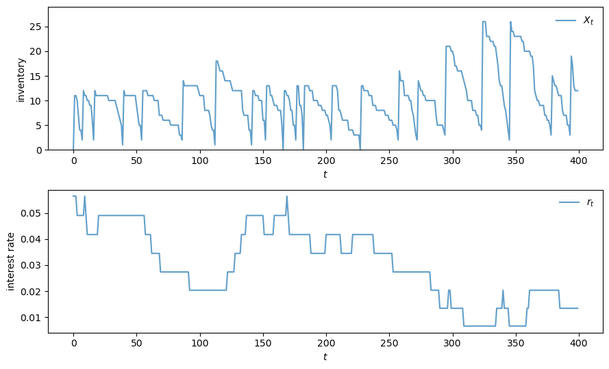
Here’s code to generate a plot.

def plot_ts(ts_length=400, fontsize=10):
    X, Z = sim_inventories(ts_length)
    fig, axes = plt.subplots(2, 1, figsize=(9, 5.5))

    ax = axes[0]
    ax.plot(X, label=r"$X_t$", alpha=0.7)
    ax.set_xlabel(r"$t$", fontsize=fontsize)
    ax.set_ylabel("inventory", fontsize=fontsize)
    ax.legend(fontsize=fontsize, frameon=False)
    ax.set_ylim(0, np.max(X)+3)

    # calculate interest rate from discount factors
    r = (1 / Z) - 1

    ax = axes[1]
    ax.plot(r, label=r"$r_t$", alpha=0.7)
    ax.set_xlabel(r"$t$", fontsize=fontsize)
    ax.set_ylabel("interest rate", fontsize=fontsize)
    ax.legend(fontsize=fontsize, frameon=False)

    plt.tight_layout()
    plt.show()

Let’s take a look.

plot_ts()

_images/05cd35f174fc4dfd15d0f23e0f5affcd74bc0fc39d0f13624e6365273183305f.png