5. Inventory Dynamics#
GPU
This lecture was built using a machine with access to a GPU — although it will also run without one.
Google Colab has a free tier with GPUs that you can access as follows:
Click on the “play” icon top right
Select Colab
Set the runtime environment to include a GPU
5.1. Overview#
This lecture explores the inventory dynamics of a firm using so-called s-S inventory control.
Loosely speaking, this means that the firm
waits until inventory falls below some value \(s\)
and then restocks up to level \(S\) (or, in some models, restocks with a bulk order of \(S\) units).
We will be interested in the distribution of the associated Markov process, which can be thought of as cross-sectional distributions of inventory levels across a large number of firms, all of which
evolve independently and
have the same dynamics.
Note that we also studied this model in a separate lecture, using Numba.
Here we study the same problem using JAX.
We will use the following imports:
import matplotlib.pyplot as plt
import numpy as np
import jax
import jax.numpy as jnp
from jax import random, lax
from typing import NamedTuple
from time import time
Here’s a description of our GPU:
!nvidia-smi
Thu Jul  9 05:40:36 2026
+-----------------------------------------------------------------------------------------+
| NVIDIA-SMI 580.105.08             Driver Version: 580.105.08     CUDA Version: 13.0     |
+-----------------------------------------+------------------------+----------------------+
| GPU  Name                 Persistence-M | Bus-Id          Disp.A | Volatile Uncorr. ECC |
| Fan  Temp   Perf          Pwr:Usage/Cap |           Memory-Usage | GPU-Util  Compute M. |
|                                         |                        |               MIG M. |
|=========================================+========================+======================|
|   0  Tesla T4                       On  |   00000000:00:1E.0 Off |                    0 |
| N/A   39C    P0             26W /   70W |       0MiB /  15360MiB |      0%      Default |
|                                         |                        |                  N/A |
+-----------------------------------------+------------------------+----------------------+

+-----------------------------------------------------------------------------------------+
| Processes:                                                                              |
|  GPU   GI   CI              PID   Type   Process name                        GPU Memory |
|        ID   ID                                                               Usage      |
|=========================================================================================|
|  No running processes found                                                             |
+-----------------------------------------------------------------------------------------+
5.2. Sample paths#
Consider a firm with inventory \(X_t\).
The firm waits until \(X_t \leq s\) and then restocks up to \(S\) units.
It faces stochastic demand \(\{ D_t \}\), which we assume is IID across time and firms.
With notation \(a^+ := \max\{a, 0\}\), inventory dynamics can be written as
In what follows, we will assume that each \(D_t\) is lognormal, so that
where \(\mu\) and \(\sigma\) are parameters and \(\{Z_t\}\) is IID and standard normal.
Here’s a namedtuple that stores parameters.
class ModelParameters(NamedTuple):
    s: int = 10
    S: int = 100
    μ: float = 1.0
    σ: float = 0.5
5.3. Cross-sectional distributions#
Now let’s look at the marginal distribution \(\psi_T\) of \(X_T\) for some fixed \(T\).
The probability distribution \(\psi_T\) is the time \(T\) distribution of firm inventory levels implied by the model.
We will approximate this distribution by
fixing \(n\) to be some large number, indicating the number of firms in the simulation,
fixing \(T\), the time period we are interested in,
generating \(n\) independent draws from some fixed distribution \(\psi_0\) that gives the initial cross-section of inventories for the \(n\) firms, and
shifting this distribution forward in time \(T\) periods, updating each firm \(T\) times via the dynamics described above (independent of other firms).
We will then visualize \(\psi_T\) by histogramming the cross-section.
We will use the following code to update the cross-section of firms by one period.
@jax.jit
def update_cross_section(params: ModelParameters,
                         X_vec: jnp.ndarray,
                         D: jnp.ndarray) -> jnp.ndarray:
    """
    Update by one period a cross-section of firms with inventory levels given by
    X_vec, given the vector of demand shocks in D. Here D[i] is the demand shock
    for firm i with current inventory X_vec[i].

    """
    # Unpack
    s, S = params.s, params.S
    # Restock if the inventory is below the threshold
    X_new = jnp.where(X_vec <= s,
                      jnp.maximum(S - D, 0),
                      jnp.maximum(X_vec - D, 0))
    return X_new
5.3.1. For loop version#
Now we provide code to compute the cross-sectional distribution \(\psi_T\) given some initial distribution \(\psi_0\) and a positive integer \(T\).
In this code we use an ordinary Python for loop to step forward through time
(Below we will squeeze out more speed by compiling the outer loop as well as the update rule.)
In the code below, the initial distribution \(\psi_0\) takes all firms to have
initial inventory x_init.
def project_cross_section(params: ModelParameters,
                          x_init: jnp.ndarray,
                          T: int,
                          key: jnp.ndarray,
                          num_firms: int = 50_000) -> jnp.ndarray:
    # Set up initial distribution
    X_vec = jnp.full((num_firms, ), x_init)
    # Loop
    for i in range(T):
        key, subkey = random.split(key)
        Z = random.normal(subkey, shape=(num_firms, ))
        D = jnp.exp(params.μ + params.σ * Z)

        X_vec = update_cross_section(params, X_vec, D)

    return X_vec
We’ll use the following specification
params = ModelParameters()
x_init = 50
T = 500
# Initialize random number generator
key = random.key(10)
Let’s look at the timing.
start_time = time()
X_vec = project_cross_section(
    params, x_init, T, key).block_until_ready()
end_time = time()
print(f"Elapsed time: {(end_time - start_time) * 1000:.6f} ms")
Elapsed time: 1151.151180 ms
Let’s run again to eliminate compile time.
start_time = time()
X_vec = project_cross_section(
    params, x_init, T, key).block_until_ready()
end_time = time()
print(f"Elapsed time: {(end_time - start_time) * 1000:.6f} ms")
Elapsed time: 394.858122 ms
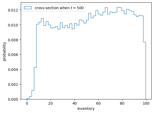
Here’s a histogram of inventory levels at time \(T\).
fig, ax = plt.subplots()
ax.hist(X_vec, bins=50,
        density=True,
        histtype='step',
        label=f'cross-section when $t = {T}$')
ax.set_xlabel('inventory')
ax.set_ylabel('probability')
ax.legend()
plt.show()
5.3.2. Compiling the outer loop#
Now let’s see if we can gain some speed by compiling the outer loop, which steps through the time dimension.
We will do this using jax.jit and a fori_loop, which is a compiler-ready version of a for loop provided by JAX.
def project_cross_section_fori(
        params: ModelParameters,
        x_init: jnp.ndarray,
        T: int,
        key: jnp.ndarray,
        num_firms: int = 50_000
    ) -> jnp.ndarray:

    s, S, μ, σ = params.s, params.S, params.μ, params.σ
    X = jnp.full((num_firms, ), x_init)

    # Define the function for each update
    def fori_update(t, loop_state):
        # Unpack
        X, key = loop_state
        # Draw shocks using key
        key, subkey = random.split(key)
        Z = random.normal(subkey, shape=(num_firms,))
        D = jnp.exp(μ + σ * Z)
        # Update X
        X = jnp.where(X <= s,
                  jnp.maximum(S - D, 0),
                  jnp.maximum(X - D, 0))
        return X, key

    # Loop t from 0 to T, applying fori_update each time.
    initial_loop_state = X, key
    X, key = lax.fori_loop(0, T, fori_update, initial_loop_state)
    return X

# Compile taking T and num_firms as static (changes trigger recompile)
project_cross_section_fori = jax.jit(
    project_cross_section_fori, static_argnums=(2, 4))
Let’s see how fast this runs with compile time.
start_time = time()
X_vec = project_cross_section_fori(
        params, x_init, T, key).block_until_ready()
end_time = time()
print(f"Elapsed time: {(end_time - start_time) * 1000:.6f} ms")
Elapsed time: 512.337685 ms
And let’s see how fast it runs without compile time.
start_time = time()
X_vec = project_cross_section_fori(
        params, x_init, T, key).block_until_ready()
end_time = time()
print(f"Elapsed time: {(end_time - start_time) * 1000:.6f} ms")
Elapsed time: 9.281158 ms
Compared to the original version with a pure Python outer loop, we have produced a nontrivial speed gain.
This is due to the fact that we have compiled the entire sequence of operations.
5.4. Distribution dynamics#
Next let’s take a look at how the distribution sequence evolves over time.
We will go back to using ordinary Python for loops.
Here is code that repeatedly shifts the cross-section forward while
recording the cross-section at the dates in sample_dates.
def shift_forward_and_sample(x_init, params, sample_dates,
                        key, num_firms=50_000, sim_length=750):

    X = res = jnp.full((num_firms, ), x_init)

    # Use for loop to update X and collect samples
    for i in range(sim_length):
        key, subkey = random.split(key)
        Z = random.normal(subkey, shape=(num_firms, ))
        D = jnp.exp(params.μ + params.σ * Z)

        X = update_cross_section(params, X, D)

        # draw a sample at the sample dates
        if (i+1 in sample_dates):
          res = jnp.vstack((res, X))

    return res[1:]
Let’s test it
x_init = 50
num_firms = 10_000
sample_dates = 10, 50, 250, 500, 750
key = random.key(10)

X = shift_forward_and_sample(
    x_init, params, sample_dates, key).block_until_ready()
Let’s plot the output.
fig, ax = plt.subplots()

for i, date in enumerate(sample_dates):
    ax.hist(X[i, :], bins=50,
            density=True,
            histtype='step',
            label=f'cross-section when $t = {date}$')

ax.set_xlabel('inventory')
ax.set_ylabel('probability')
ax.legend()
plt.show()
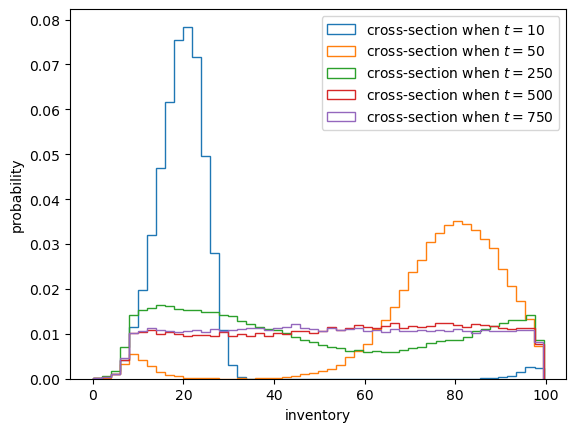
This model for inventory dynamics is asymptotically stationary, with a unique stationary distribution.
In particular, the sequence of marginal distributions \(\{\psi_t\}\) converges to a unique limiting distribution that does not depend on initial conditions.
Intuitively, demand shocks repeatedly push inventories downward, while the threshold rule returns low-inventory firms to a common upper inventory level, so the process gradually forgets its initial condition.
Although we will not prove this here, we can see it in the simulation above.
By \(t=500\) or \(t=750\) the distributions are barely changing.
If you test a few different initial conditions, you will see that they do not affect long-run outcomes.
5.5. Restock frequency#
As an exercise, let’s study the probability that firms need to restock over a given time period.
In the exercise, we will
set the starting stock level to \(X_0 = 70\) and
calculate the proportion of firms that need to order twice or more in the first 50 periods.
This proportion approximates the probability of the event when the sample size is large.
5.5.1. For loop version#
We start with an easier for loop implementation
# Define a jitted function for each update
@jax.jit
def update_stock(n_restock, X, params, D):
    n_restock = jnp.where(X <= params.s,
                          n_restock + 1,
                          n_restock)
    X = jnp.where(X <= params.s,
                  jnp.maximum(params.S - D, 0),
                  jnp.maximum(X - D, 0))
    return n_restock, X

def compute_freq(params, key,
                 x_init=70,
                 sim_length=50,
                 num_firms=1_000_000):

    # Prepare initial arrays
    X = jnp.full((num_firms, ), x_init)

    # Stack the restock counter on top of the inventory
    n_restock = jnp.zeros((num_firms, ))

    # Use a for loop to perform the calculations on all states
    for i in range(sim_length):
        key, subkey = random.split(key)
        Z = random.normal(subkey, shape=(num_firms, ))
        D = jnp.exp(params.μ + params.σ * Z)
        n_restock, X = update_stock(
            n_restock, X, params, D)

    return jnp.mean(n_restock > 1, axis=0)
key = random.key(27)

start_time = time()
freq = compute_freq(params, key).block_until_ready()
end_time = time()
print(f"Elapsed time: {(end_time - start_time) * 1000:.6f} ms")
Elapsed time: 805.397749 ms
We run the code again to get rid of compile time.
start_time = time()
freq = compute_freq(params, key).block_until_ready()
end_time = time()
print(f"Elapsed time: {(end_time - start_time) * 1000:.6f} ms")
Elapsed time: 45.172215 ms
print(f"Frequency of at least two stock outs = {freq}")
Frequency of at least two stock outs = 0.44729599356651306
Exercise 5.1
Write a fori_loop version of the last function. See if you can increase the
speed while generating a similar answer.
Solution
Here is a lax.fori_loop version that JIT compiles the whole function
def compute_freq(params, key,
                 x_init=70,
                 sim_length=50,
                 num_firms=1_000_000):

    s, S, μ, σ = params.s, params.S, params.μ, params.σ
    # Prepare initial arrays
    X = jnp.full((num_firms, ), x_init)
    Z = random.normal(key, shape=(sim_length, num_firms))
    D = jnp.exp(μ + σ * Z)

    # Stack the restock counter on top of the inventory
    restock_count = jnp.zeros((num_firms, ))
    Xs = (X, restock_count)

    # Define the function for each update
    def update_cross_section(i, Xs):
        # Separate the inventory and restock counter
        x, restock_count = Xs[0], Xs[1]
        restock_count = jnp.where(x <= s,
                                restock_count + 1,
                                restock_count)
        x = jnp.where(x <= s,
                      jnp.maximum(S - D[i], 0),
                      jnp.maximum(x - D[i], 0))

        Xs = (x, restock_count)
        return Xs

    # Use lax.fori_loop to perform the calculations on all states
    X_final = lax.fori_loop(0, sim_length, update_cross_section, Xs)

    return jnp.mean(X_final[1] > 1)

# Compile taking sim_length and num_firms as static (changes trigger recompile)
compute_freq = jax.jit(compute_freq, static_argnums=(3, 4))
Note the time the routine takes to run, as well as the output
start_time = time()
freq = compute_freq(params, key).block_until_ready()
end_time = time()
print(f"Elapsed time: {(end_time - start_time) * 1000:.6f} ms")
Elapsed time: 427.071095 ms
We run the code again to eliminate the compile time.
start_time = time()
freq = compute_freq(params, key).block_until_ready()
end_time = time()
print(f"Elapsed time: {(end_time - start_time) * 1000:.6f} ms")
Elapsed time: 8.063793 ms
print(f"Frequency of at least two stock outs = {freq}")
Frequency of at least two stock outs = 0.4476909935474396