3. Adventures with Autodiff#
GPU
This lecture was built using a machine with access to a GPU — although it will also run without one.
Google Colab has a free tier with GPUs that you can access as follows:
Click on the “play” icon top right
Select Colab
Set the runtime environment to include a GPU
3.1. Overview#
This lecture gives a brief introduction to automatic differentiation using Google JAX.
Automatic differentiation is one of the key elements of modern machine learning and artificial intelligence.
As such it has attracted a great deal of investment and there are several powerful implementations available.
One of the best of these is the automatic differentiation routines contained in JAX.
While other software packages also offer this feature, the JAX version is particularly powerful because it integrates so well with other core components of JAX (e.g., JIT compilation and parallelization).
As we will see in later lectures, automatic differentiation can be used not only for AI but also for many problems faced in mathematical modeling, such as multi-dimensional nonlinear optimization and root-finding problems.
We need the following imports
import jax
import jax.numpy as jnp
import matplotlib.pyplot as plt
import numpy as np
Checking for a GPU:
!nvidia-smi
Thu Jul  9 05:39:27 2026
+-----------------------------------------------------------------------------------------+
| NVIDIA-SMI 580.105.08             Driver Version: 580.105.08     CUDA Version: 13.0     |
+-----------------------------------------+------------------------+----------------------+
| GPU  Name                 Persistence-M | Bus-Id          Disp.A | Volatile Uncorr. ECC |
| Fan  Temp   Perf          Pwr:Usage/Cap |           Memory-Usage | GPU-Util  Compute M. |
|                                         |                        |               MIG M. |
|=========================================+========================+======================|
|   0  Tesla T4                       On  |   00000000:00:1E.0 Off |                    0 |
| N/A   35C    P0             25W /   70W |       0MiB /  15360MiB |      0%      Default |
|                                         |                        |                  N/A |
+-----------------------------------------+------------------------+----------------------+

+-----------------------------------------------------------------------------------------+
| Processes:                                                                              |
|  GPU   GI   CI              PID   Type   Process name                        GPU Memory |
|        ID   ID                                                               Usage      |
|=========================================================================================|
|  No running processes found                                                             |
+-----------------------------------------------------------------------------------------+
3.2. What is automatic differentiation?#
Autodiff is a technique for calculating derivatives on a computer.
3.2.1. Autodiff is not finite differences#
The derivative of \(f(x) = \exp(2x)\) is
A computer that doesn’t know how to take derivatives might approximate this with the finite difference ratio
where \(h\) is a small positive number.
def f(x):
    "Original function."
    return np.exp(2 * x)

def f_prime(x):
    "True derivative."
    return 2 * np.exp(2 * x)

def Df(x, h=0.1):
    "Approximate derivative (finite difference)."
    return (f(x + h) - f(x))/h

x_grid = np.linspace(-2, 1, 200)
fig, ax = plt.subplots()
ax.plot(x_grid, f_prime(x_grid), label="$f'$")
ax.plot(x_grid, Df(x_grid), label="$Df$")
ax.legend()
plt.show()
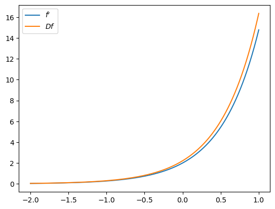
This kind of numerical derivative is often inaccurate and unstable.
One reason is that
Small numbers in the numerator and denominator causes rounding errors.
The situation is exponentially worse in high dimensions / with higher order derivatives
3.2.2. Autodiff is not symbolic calculus#
Symbolic calculus tries to use rules for differentiation to produce a single closed-form expression representing a derivative.
from sympy import symbols, diff

m, a, b, x = symbols('m a b x')
f_x = (a*x + b)**m
f_x.diff((x, 6))  # 6-th order derivative
Symbolic calculus is not well suited to high performance computing.
One disadvantage is that symbolic calculus cannot differentiate through control flow.
Also, using symbolic calculus might involve redundant calculations.
For example, consider
If we evaluate at \(x\), then we evalute \(f(x)\) and \(g(x)\) twice each.
Also, computing \(f'(x)\) and \(f(x)\) might involve similar terms (e.g., \((f(x) = \exp(2x)' \implies f'(x) = 2f(x)\)) but this is not exploited in symbolic algebra.
3.2.3. Autodiff#
Autodiff produces functions that evaluates derivatives at numerical values passed in by the calling code, rather than producing a single symbolic expression representing the entire derivative.
Derivatives are constructed by breaking calculations into component parts via the chain rule.
The chain rule is applied until the point where the terms reduce to primitive functions that the program knows how to differentiate exactly (addition, subtraction, exponentiation, sine and cosine, etc.)
3.3. Some experiments#
Let’s start with some real-valued functions on \(\mathbb R\).
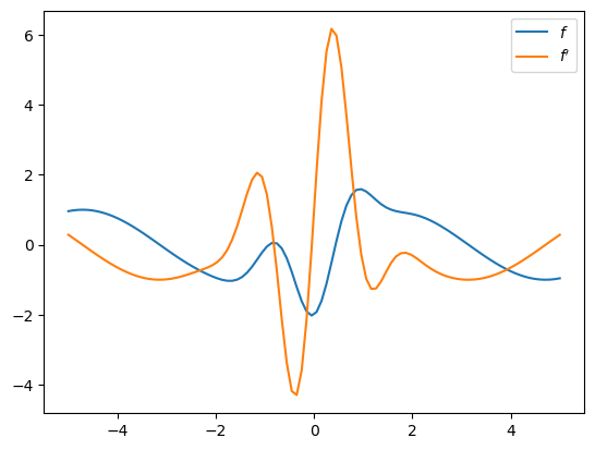
3.3.1. A differentiable function#
Let’s test JAX’s auto diff with a relatively simple function.
def f(x):
    return jnp.sin(x) - 2 * jnp.cos(3 * x) * jnp.exp(- x**2)
We use grad to compute the gradient of a real-valued function:
f_prime = jax.grad(f)
Let’s plot the result:
x_grid = jnp.linspace(-5, 5, 100)
fig, ax = plt.subplots()
ax.plot(x_grid, [f(x) for x in x_grid], label="$f$")
ax.plot(x_grid, [f_prime(x) for x in x_grid], label="$f'$")
ax.legend()
plt.show()
3.3.2. Absolute value function#
What happens if the function is not differentiable?
def f(x):
    return jnp.abs(x)
f_prime = jax.grad(f)
fig, ax = plt.subplots()
ax.plot(x_grid, [f(x) for x in x_grid], label="$f$")
ax.plot(x_grid, [f_prime(x) for x in x_grid], label="$f'$")
ax.legend()
plt.show()
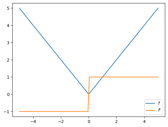
At the nondifferentiable point \(0\), jax.grad returns the right derivative:
f_prime(0.0)
Array(1., dtype=float32, weak_type=True)
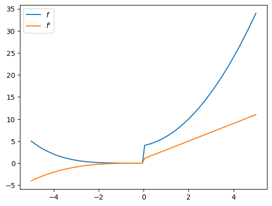
3.3.3. Differentiating through control flow#
Let’s try differentiating through some loops and conditions.
def f(x):
    def f1(x):
        for i in range(2):
            x *= 0.2 * x
        return x
    def f2(x):
        x = sum((x**i + i) for i in range(3))
        return x
    y = f1(x) if x < 0 else f2(x)
    return y
f_prime = jax.grad(f)
x_grid = jnp.linspace(-5, 5, 100)
fig, ax = plt.subplots()
ax.plot(x_grid, [f(x) for x in x_grid], label="$f$")
ax.plot(x_grid, [f_prime(x) for x in x_grid], label="$f'$")
ax.legend()
plt.show()
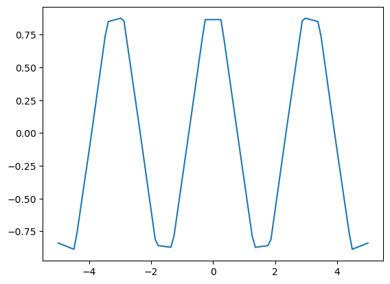
3.3.4. Differentiating through a linear interpolation#
We can differentiate through linear interpolation, even though the function is not smooth:
n = 20
xp = jnp.linspace(-5, 5, n)
yp = jnp.cos(2 * xp)

fig, ax = plt.subplots()
ax.plot(x_grid, jnp.interp(x_grid, xp, yp))
plt.show()
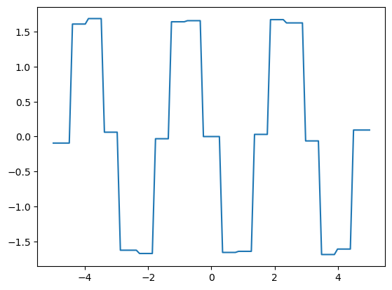
f_prime = jax.grad(jnp.interp)
f_prime_vec = jax.vmap(f_prime, in_axes=(0, None, None))
fig, ax = plt.subplots()
ax.plot(x_grid, f_prime_vec(x_grid, xp, yp))
plt.show()
3.4. Gradient Descent#
Let’s try implementing gradient descent.
As a simple application, we’ll use gradient descent to solve for the OLS parameter estimates in simple linear regression.
3.4.1. A function for gradient descent#
Here’s an implementation of gradient descent.
def grad_descent(f,       # Function to be minimized
                 args,    # Extra arguments to the function
                 x0,      # Initial condition
                 λ=0.1,   # Initial learning rate
                 tol=1e-5,
                 max_iter=1_000):
    """
    Minimize the function f via gradient descent, starting from guess x0.

    The learning rate is computed according to the Barzilai-Borwein method.

    """

    f_grad = jax.grad(f)
    x = jnp.array(x0)
    df = f_grad(x, args)
    ϵ = tol + 1
    i = 0
    while ϵ > tol and i < max_iter:
        new_x = x - λ * df
        new_df = f_grad(new_x, args)
        Δx = new_x - x
        Δdf = new_df - df
        λ = jnp.abs(Δx @ Δdf) / (Δdf @ Δdf)
        ϵ = jnp.max(jnp.abs(Δx))
        x, df = new_x, new_df
        i += 1

    return x
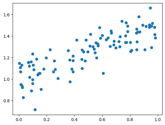
3.4.2. Simulated data#
We’re going to test our gradient descent function my minimizing a sum of least squares in a regression problem.
Let’s generate some simulated data:
n = 100
key = jax.random.key(1234)
x = jax.random.uniform(key, (n,))

α, β, σ = 0.5, 1.0, 0.1  # Set the true intercept and slope.
key, subkey = jax.random.split(key)
ϵ = jax.random.normal(subkey, (n,))

y = α * x + β + σ * ϵ
fig, ax = plt.subplots()
ax.scatter(x, y)
plt.show()
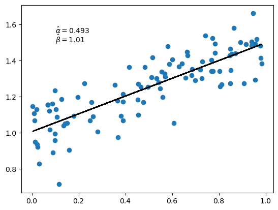
Let’s start by calculating the estimated slope and intercept using closed form solutions.
mx = x.mean()
my = y.mean()
α_hat = jnp.sum((x - mx) * (y - my)) / jnp.sum((x - mx)**2)
β_hat = my - α_hat * mx
α_hat, β_hat
(Array(0.49340868, dtype=float32), Array(1.0055456, dtype=float32))
fig, ax = plt.subplots()
ax.scatter(x, y)
ax.plot(x, α_hat * x + β_hat, 'k-')
ax.text(0.1, 1.55, rf'$\hat \alpha = {α_hat:.3}$')
ax.text(0.1, 1.50, rf'$\hat \beta = {β_hat:.3}$')
plt.show()
3.4.3. Minimizing squared loss by gradient descent#
Let’s see if we can get the same values with our gradient descent function.
First we set up the least squares loss function.
@jax.jit
def loss(params, data):
    a, b = params
    x, y = data
    return jnp.sum((y - a * x - b)**2)
Now we minimize it:
p0 = jnp.zeros(2)  # Initial guess for α, β
data = x, y
α_hat, β_hat = grad_descent(loss, data, p0)
Let’s plot the results.
fig, ax = plt.subplots()
x_grid = jnp.linspace(0, 1, 100)
ax.scatter(x, y)
ax.plot(x_grid, α_hat * x_grid + β_hat, 'k-', alpha=0.6)
ax.text(0.1, 1.55, rf'$\hat \alpha = {α_hat:.3}$')
ax.text(0.1, 1.50, rf'$\hat \beta = {β_hat:.3}$')
plt.show()
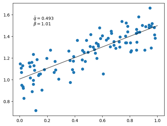
Notice that we get the same estimates as we did from the closed form solutions.
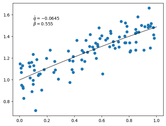
3.4.4. Adding a squared term#
Now let’s try fitting a second order polynomial.
Here’s our new loss function.
@jax.jit
def loss(params, data):
    a, b, c = params
    x, y = data
    return jnp.sum((y - a * x**2 - b * x - c)**2)
Now we’re minimizing in three dimensions.
Let’s try it.
p0 = jnp.zeros(3)
α_hat, β_hat, γ_hat = grad_descent(loss, data, p0)

fig, ax = plt.subplots()
ax.scatter(x, y)
ax.plot(x_grid, α_hat * x_grid**2 + β_hat * x_grid + γ_hat, 'k-', alpha=0.6)
ax.text(0.1, 1.55, rf'$\hat \alpha = {α_hat:.3}$')
ax.text(0.1, 1.50, rf'$\hat \beta = {β_hat:.3}$')
plt.show()
3.5. Exercises#
Exercise 3.1
The function jnp.polyval evaluates polynomials.
For example, if len(p) is 3, then jnp.polyval(p, x) returns
Use this function for polynomial regression.
The (empirical) loss becomes
Set \(k=4\) and set the initial guess of params to jnp.zeros(k).
Use gradient descent to find the array params that minimizes the loss
function and plot the result (following the examples above).
Solution
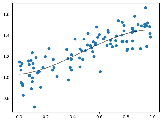
Here’s one solution.
def loss(params, data):
    x, y = data
    return jnp.sum((y - jnp.polyval(params, x))**2)
k = 4
p0 = jnp.zeros(k)
p_hat = grad_descent(loss, data, p0)
print('Estimated parameter vector:')
print(p_hat)
print('\n\n')

fig, ax = plt.subplots()
ax.scatter(x, y)
ax.plot(x_grid, jnp.polyval(p_hat, x_grid), 'k-', alpha=0.6)
plt.show()
Estimated parameter vector:
[-0.76444525  1.0770515   0.11147378  1.0265538 ]