5. Kesten Processes and Firm Dynamics#

GPU

This lecture was built using a machine with JAX installed and access to a GPU.

To run this lecture on Google Colab, click on the “play” icon top right, select Colab, and set the runtime environment to include a GPU.

To run this lecture on your own machine, you need to install Google JAX.

In addition to JAX and Anaconda, this lecture will need the following libraries:

!pip install quantecon

5.1. Overview#

This lecture describes Kesten processes, which are an important class of stochastic processes, and an application of firm dynamics.

The lecture draws on an earlier QuantEcon lecture, which uses Numba to accelerate the computations.

In that earlier lecture you can find a more detailed discussion of the concepts involved.

This lecture focuses on implementing the same computations in JAX.

Let’s start with some imports:

import matplotlib.pyplot as plt
import quantecon as qe
import jax
import jax.numpy as jnp
from jax import random
from jax import lax

Let’s check the GPU we are running

!nvidia-smi

/opt/conda/envs/quantecon/lib/python3.11/pty.py:89: RuntimeWarning: os.fork() was called. os.fork() is incompatible with multithreaded code, and JAX is multithreaded, so this will likely lead to a deadlock.
  pid, fd = os.forkpty()

Tue May  7 07:29:29 2024       
+-----------------------------------------------------------------------------+
| NVIDIA-SMI 470.182.03   Driver Version: 470.182.03   CUDA Version: 12.3     |
|-------------------------------+----------------------+----------------------+
| GPU  Name        Persistence-M| Bus-Id        Disp.A | Volatile Uncorr. ECC |
| Fan  Temp  Perf  Pwr:Usage/Cap|         Memory-Usage | GPU-Util  Compute M. |
|                               |                      |               MIG M. |
|===============================+======================+======================|

|   0  Tesla V100-SXM2...  Off  | 00000000:00:1E.0 Off |                    0 |
| N/A   31C    P0    37W / 300W |      0MiB / 16160MiB |      2%      Default |
|                               |                      |                  N/A |
+-------------------------------+----------------------+----------------------+
                                                                               
+-----------------------------------------------------------------------------+
| Processes:                                                                  |
|  GPU   GI   CI        PID   Type   Process name                  GPU Memory |
|        ID   ID                                                   Usage      |
|=============================================================================|
|  No running processes found                                                 |
+-----------------------------------------------------------------------------+

5.2. Kesten processes#

A Kesten process is a stochastic process of the form

(5.1)#\[X_{t+1} = a_{t+1} X_t + \eta_{t+1}\]

where \(\{a_t\}_{t \geq 1}\) and \(\{\eta_t\}_{t \geq 1}\) are IID sequences.

We are interested in the dynamics of \(\{X_t\}_{t \geq 0}\) when \(X_0\) is given.

We will focus on the nonnegative scalar case, where \(X_t\) takes values in \(\mathbb R_+\).

In particular, we will assume that

the initial condition \(X_0\) is nonnegative,
\(\{a_t\}_{t \geq 1}\) is a nonnegative IID stochastic process and
\(\{\eta_t\}_{t \geq 1}\) is another nonnegative IID stochastic process, independent of the first.

5.2.1. Application: firm dynamics#

In this section we apply Kesten process theory to the study of firm dynamics.

5.2.1.1. Gibrat’s law#

It was postulated many years ago by Robert Gibrat that firm size evolves according to a simple rule whereby size next period is proportional to current size.

This is now known as Gibrat’s law of proportional growth.

We can express this idea by stating that a suitably defined measure \(s_t\) of firm size obeys

(5.2)#\[\frac{s_{t+1}}{s_t} = a_{t+1}\]

for some positive IID sequence \(\{a_t\}\).

Subsequent empirical research has shown that this specification is not accurate, particularly for small firms.

However, we can get close to the data by modifying (5.2) to

(5.3)#\[s_{t+1} = a_{t+1} s_t + b_{t+1}\]

where \(\{a_t\}\) and \(\{b_t\}\) are both IID and independent of each other.

We now study the implications of this specification.

5.2.1.2. Heavy tails#

If the conditions of the Kesten–Goldie Theorem are satisfied, then (5.3) implies that the firm size distribution will have Pareto tails.

This matches empirical findings across many data sets.

But there is another unrealistic aspect of the firm dynamics specified in (5.3) that we need to address: it ignores entry and exit.

In any given period and in any given market, we observe significant numbers of firms entering and exiting the market.

In this setting, firm dynamics can be expressed as

(5.4)#\[ s_{t+1} = e_{t+1} \mathbb{1}\{s_t < \bar s\} + (a_{t+1} s_t + b_{t+1}) \mathbb{1}\{s_t \geq \bar s\}\]

The motivation behind and interpretation of (5.4) can be found in our earlier Kesten process lecture.

What can we say about dynamics?

Although (5.4) is not a Kesten process, it does update in the same way as a Kesten process when \(s_t\) is large.

So perhaps its stationary distribution still has Pareto tails?

We can investigate this question via simulation and rank-size plots.

The approach will be to

generate \(M\) draws of \(s_T\) when \(M\) and \(T\) are large and
plot the largest 1,000 of the resulting draws in a rank-size plot.

(The distribution of \(s_T\) will be close to the stationary distribution when \(T\) is large.)

In the simulation, we assume that each of \(a_t, b_t\) and \(e_t\) is lognormal.

Here’s code to update a cross-section of firms according to the dynamics in (5.4).

@jax.jit
def update_s(s, s_bar, a_random, b_random, e_random):
    exp_a = jnp.exp(a_random)
    exp_b = jnp.exp(b_random)
    exp_e = jnp.exp(e_random)

    s = jnp.where(s < s_bar,
                  exp_e,
                  exp_a * s + exp_b)

    return s

Now we write a for loop that repeatedly calls this function, to push a cross-section of firms forward in time.

For sufficiently large T, the cross-section it returns (the cross-section at time T) corresponds to firm size distribution in (approximate) equilibrium.

def generate_draws(M=1_000_000,
                   μ_a=-0.5,
                   σ_a=0.1,
                   μ_b=0.0,
                   σ_b=0.5,
                   μ_e=0.0,
                   σ_e=0.5,
                   s_bar=1.0,
                   T=500,
                   s_init=1.0,
                   seed=123):

    key = random.PRNGKey(seed)

    # Initialize the array of s values with the initial value
    s = jnp.full((M, ), s_init)

    # Perform updates on s for time t
    for t in range(T):
        keys = random.split(key, 3)
        a_random = μ_a + σ_a * random.normal(keys[0], (M, ))
        b_random = μ_b + σ_b * random.normal(keys[1], (M, ))
        e_random = μ_e + σ_e * random.normal(keys[2], (M, ))

        s = update_s(s, s_bar, a_random, b_random, e_random)
        
        # Generate new key for the next iteration
        key = random.fold_in(key, t)

    return s

%time data = generate_draws().block_until_ready()

CPU times: user 4.02 s, sys: 2.27 s, total: 6.29 s
Wall time: 3.77 s

Running the above function again so we can see the speed with and without compile time.

%time data = generate_draws().block_until_ready()

CPU times: user 3.84 s, sys: 807 ms, total: 4.65 s
Wall time: 1.96 s

Notice that we do not JIT-compile the for loops, since

acceleration of the outer loop makes little difference terms of compute time and
compiling the outer loop is often very slow.

Let’s produce the rank-size plot and check the distribution:

fig, ax = plt.subplots()

rank_data, size_data = qe.rank_size(data, c=0.01)
ax.loglog(rank_data, size_data, 'o', markersize=3.0, alpha=0.5)
ax.set_xlabel("log rank")
ax.set_ylabel("log size")

plt.show()

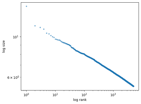
_images/983d57069e6fb306e037e6f5abd5114ffe3f2f3d384f9e3d87d7c762c5841c96.png

The plot produces a straight line, consistent with a Pareto tail.

5.2.1.3. Alternative implementation with `lax.fori_loop`#

If the time horizon is not too large, we can try to further accelerate our code by replacing the for loop with lax.fori_loop.

Note, however, that

as mentioned above, there is not much speed gain in accelerating outer loops,
lax.fori_loop has a more complicated syntax, and, most importantly,
the lax.fori_loop implementation consumes far more memory, as we need to have to store large matrices of random draws

Hence the code below will fail due to out-of-memory errors when T and M are large.

Here is the lax.fori_loop version:

@jax.jit
def generate_draws_lax(μ_a=-0.5,
                       σ_a=0.1,
                       μ_b=0.0,
                       σ_b=0.5,
                       μ_e=0.0,
                       σ_e=0.5,
                       s_bar=1.0,
                       T=500,
                       M=500_000,
                       s_init=1.0,
                       seed=123):

    key = random.PRNGKey(seed)
    keys = random.split(key, 3)
    
    # Generate random draws and initial values
    a_random = μ_a + σ_a * random.normal(keys[0], (T, M))
    b_random = μ_b + σ_b * random.normal(keys[1], (T, M))
    e_random = μ_e + σ_e * random.normal(keys[2], (T, M))
    s = jnp.full((M, ), s_init)

    # Define the function for each update
    def update_s(i, s):
        a, b, e = a_random[i], b_random[i], e_random[i]
        s = jnp.where(s < s_bar,
                      jnp.exp(e),
                      jnp.exp(a) * s + jnp.exp(b))
        return s

    # Use lax.scan to perform the calculations on all states
    s_final = lax.fori_loop(0, T, update_s, s)
    return s_final

%time data = generate_draws_lax().block_until_ready()

CPU times: user 400 ms, sys: 0 ns, total: 400 ms
Wall time: 398 ms

In this case, M is small enough for the code to run and we see some speed gain over the for loop implementation:

%time data = generate_draws_lax().block_until_ready()

CPU times: user 3.61 ms, sys: 0 ns, total: 3.61 ms
Wall time: 34.8 ms

Here we produce the same rank-size plot:

fig, ax = plt.subplots()

rank_data, size_data = qe.rank_size(data, c=0.01)
ax.loglog(rank_data, size_data, 'o', markersize=3.0, alpha=0.5)
ax.set_xlabel("log rank")
ax.set_ylabel("log size")

plt.show()

_images/1e7de32e53634e0050197d9ea1a340021f12391da008b2b26dd9593eedff01a4.png

Let’s rerun the for loop version on smaller M to compare the speed

%time generate_draws(M=500_000).block_until_ready()

CPU times: user 4.39 s, sys: 561 ms, total: 4.96 s
Wall time: 2.24 s

Array([2.389801 , 2.2558599, 3.3113828, ..., 2.7102313, 2.5520844,
       3.4196172], dtype=float32)

We see that the lax.fori_loop version is faster than the for loop version when memory is not an issue.