6. Wealth Distribution Dynamics#

GPU

This lecture was built using a machine with JAX installed and access to a GPU.

To run this lecture on Google Colab, click on the “play” icon top right, select Colab, and set the runtime environment to include a GPU.

To run this lecture on your own machine, you need to install Google JAX.

In this lecture we examine wealth dynamics in large cross-section of agents who are subject to both

idiosyncratic shocks, which affect labor income and returns, and
an aggregate shock, which also impacts on labor income and returns

In most macroeconomic models savings and consumption are determined by optimization.

Here savings and consumption behavior is taken as given – you can plug in your favorite model to obtain savings behavior and then analyze distribution dynamics using the techniques described below.

One of our interests will be how different aspects of wealth dynamics – such as labor income and the rate of return on investments – feed into measures of inequality, such as the Gini coefficient.

In addition to JAX and Anaconda, this lecture will need the following libraries:

!pip install quantecon

We will use the following imports:

import numba
import pandas as pd
import numpy as np
import matplotlib.pyplot as plt
import quantecon as qe
import jax
import jax.numpy as jnp
from time import time

Let’s check the GPU we are running

!nvidia-smi

Thu Jun 13 04:31:18 2024       
+---------------------------------------------------------------------------------------+
| NVIDIA-SMI 535.54.03              Driver Version: 535.54.03    CUDA Version: 12.5     |
|-----------------------------------------+----------------------+----------------------+
| GPU  Name                 Persistence-M | Bus-Id        Disp.A | Volatile Uncorr. ECC |
| Fan  Temp   Perf          Pwr:Usage/Cap |         Memory-Usage | GPU-Util  Compute M. |
|                                         |                      |               MIG M. |
|=========================================+======================+======================|
|   0  Tesla T4                       On  | 00000001:00:00.0 Off |                  Off |
| N/A   58C    P8              10W /  70W |      2MiB / 16384MiB |      0%      Default |
|                                         |                      |                  N/A |
+-----------------------------------------+----------------------+----------------------+
                                                                                         
+---------------------------------------------------------------------------------------+
| Processes:                                                                            |
|  GPU   GI   CI        PID   Type   Process name                            GPU Memory |
|        ID   ID                                                             Usage      |
|=======================================================================================|
|  No running processes found                                                           |
+---------------------------------------------------------------------------------------+

6.1. Wealth dynamics#

Wealth evolves as follows:

\[ w_{t+1} = (1 + r_{t+1}) s(w_t) + y_{t+1}\]

Here

$w_t$ is wealth at time $t$ for a given household,
$r_t$ is the rate of return of financial assets,
$y_t$ is labor income and
$s(w_t)$ is savings (current wealth minus current consumption)

There is an aggregate state process

\[ z_{t+1} = a z_t + b + \sigma_z \epsilon_{t+1} \]

that affects the interest rate and labor income.

In particular, the gross interest rates obey

\[ R_t := 1 + r_t = c_r \exp(z_t) + \exp(\mu_r + \sigma_r \xi_t) \]

while

\[ y_t = c_y \exp(z_t) + \exp(\mu_y + \sigma_y \zeta_t) \]

The tuple $\{ (\epsilon_t, \xi_t, \zeta_t) \}$ is IID and standard normal in $\mathbb R^3$.

(Each household receives their own idiosyncratic shocks.)

Regarding the savings function $s$, our default model will be

(6.1)#\[s(w) = s_0 w \cdot \mathbb 1\{w \geq \hat w\}\]

where $s_0$ is a positive constant.

Thus,

for $w < \hat w$, the household saves nothing, while
for $w \geq \bar w$, the household saves a fraction $s_0$ of their wealth.

6.2. Implementation#

6.2.1. Numba implementation#

Here’s a function that collects parameters and useful constants

def create_wealth_model(w_hat=1.0,   # Savings parameter
                        s_0=0.75,    # Savings parameter
                        c_y=1.0,     # Labor income parameter
                        μ_y=1.0,     # Labor income parameter
                        σ_y=0.2,     # Labor income parameter
                        c_r=0.05,    # Rate of return parameter
                        μ_r=0.1,     # Rate of return parameter
                        σ_r=0.5,     # Rate of return parameter
                        a=0.5,       # Aggregate shock parameter
                        b=0.0,       # Aggregate shock parameter
                        σ_z=0.1):    # Aggregate shock parameter
    """
    Create a wealth model with given parameters. 

    Return a tuple model = (household_params, aggregate_params), where
    household_params collects household information and aggregate_params
    collects information relevant to the aggregate shock process.
    
    """
    # Mean and variance of z process
    z_mean = b / (1 - a)
    z_var = σ_z**2 / (1 - a**2)
    exp_z_mean = np.exp(z_mean + z_var / 2)
    # Mean of R and y processes
    R_mean = c_r * exp_z_mean + np.exp(μ_r + σ_r**2 / 2)
    y_mean = c_y * exp_z_mean + np.exp(μ_y + σ_y**2 / 2)
    # Test stability condition ensuring wealth does not diverge
    # to infinity.
    α = R_mean * s_0
    if α >= 1:
        raise ValueError("Stability condition failed.")
    # Pack values into tuples and return them
    household_params = (w_hat, s_0, c_y, μ_y, σ_y, c_r, μ_r, σ_r, y_mean)
    aggregate_params = (a, b, σ_z, z_mean, z_var)
    model = household_params, aggregate_params
    return model

Here’s a function that generates the aggregate state process

@numba.jit
def generate_aggregate_state_sequence(aggregate_params, length=100):
    a, b, σ_z, z_mean, z_var = aggregate_params 
    z = np.empty(length+1)
    z[0] = z_mean   # Initialize at z_mean
    for t in range(length):
        z[t+1] = a * z[t] + b + σ_z * np.random.randn()
    return z

Here’s a function that updates household wealth by one period, taking the current value of the aggregate shock

@numba.jit
def update_wealth(household_params, w, z):
    """
    Generate w_{t+1} given w_t and z_{t+1}.
    """
    # Unpack
    w_hat, s_0, c_y, μ_y, σ_y, c_r, μ_r, σ_r, y_mean = household_params
    # Update wealth
    y = c_y * np.exp(z) + np.exp(μ_y + σ_y * np.random.randn())
    wp = y
    if w >= w_hat:
        R = c_r * np.exp(z) + np.exp(μ_r + σ_r * np.random.randn())
        wp += R * s_0 * w
    return wp

Here’s a function to simulate the time series of wealth for an individual household

@numba.jit
def wealth_time_series(model, w_0, sim_length):
    """
    Generate a single time series of length sim_length for wealth given initial
    value w_0.  The function generates its own aggregate shock sequence.

    """
    # Unpack
    household_params, aggregate_params = model
    a, b, σ_z, z_mean, z_var = aggregate_params 
    # Initialize and update
    z = generate_aggregate_state_sequence(aggregate_params, 
                                          length=sim_length)
    w = np.empty(sim_length)
    w[0] = w_0
    for t in range(sim_length-1):
        w[t+1] = update_wealth(household_params, w[t], z[t+1])
    return w

Let’s look at the wealth dynamics of an individual household

model = create_wealth_model()
household_params, aggregate_params = model
w_hat, s_0, c_y, μ_y, σ_y, c_r, μ_r, σ_r, y_mean = household_params
a, b, σ_z, z_mean, z_var = aggregate_params 
ts_length = 200
w = wealth_time_series(model, y_mean, ts_length)

fig, ax = plt.subplots()
ax.plot(w)
plt.show()

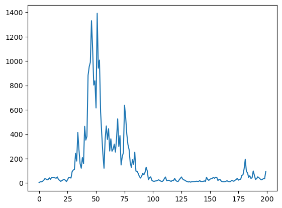
_images/5cf3b3546d0c1737c035e29cf742237c97aa030800c60afe32bbc71f0d6fc9ef.png

Notice the large spikes in wealth over time.

Such spikes are related to heavy tails in the wealth distribution, which we discuss below.

Here’s a function to simulate a cross section of households forward in time.

Note the use of parallelization to speed up computation.

@numba.jit(parallel=True)
def update_cross_section(model, w_distribution, z_sequence):
    """
    Shifts a cross-section of households forward in time

    Takes 

        * a current distribution of wealth values as w_distribution and
        * an aggregate shock sequence z_sequence

    and updates each w_t in w_distribution to w_{t+j}, where
    j = len(z_sequence).

    Returns the new distribution.

    """
    # Unpack
    household_params, aggregate_params = model

    num_households = len(w_distribution)
    new_distribution = np.empty_like(w_distribution)
    z = z_sequence

    # Update each household
    for i in numba.prange(num_households):
        w = w_distribution[i]
        for t in range(sim_length):
            w = update_wealth(household_params, w, z[t])
        new_distribution[i] = w
    return new_distribution

Parallelization works in the function above because the time path of each household can be calculated independently once the path for the aggregate state is known.

Let’s see how long it takes to shift a large cross-section of households forward 200 periods

sim_length = 200
num_households = 10_000_000
ψ_0 = np.full(num_households, y_mean)  # Initial distribution
z_sequence = generate_aggregate_state_sequence(aggregate_params,
                                               length=sim_length)
print("Generating cross-section using Numba")
start = time()
ψ_star = update_cross_section(model, ψ_0, z_sequence)
numba_with_compile = time() - start
print(f"Generated cross-section in {numba_with_compile} seconds.\n")

Generating cross-section using Numba

Generated cross-section in 56.959468126297 seconds.

We run it again to eliminate compile time.

start = time()
ψ_star = update_cross_section(model, ψ_0, z_sequence)
numba_without_compile = time() - start
print(f"Generated cross-section in {numba_without_compile} seconds.\n")

Generated cross-section in 56.71404027938843 seconds.

6.2.2. JAX implementation#

Let’s redo some of the preceding calculations using JAX and see how execution speed compares

def update_cross_section_jax(model, w_distribution, z_sequence, key):
    """
    Shifts a cross-section of households forward in time

    Takes 

        * a current distribution of wealth values as w_distribution and
        * an aggregate shock sequence z_sequence

    and updates each w_t in w_distribution to w_{t+j}, where
    j = len(z_sequence).

    Returns the new distribution.

    """
    # Unpack, simplify names
    household_params, aggregate_params = model
    w_hat, s_0, c_y, μ_y, σ_y, c_r, μ_r, σ_r, y_mean = household_params
    w = w_distribution
    n = len(w)

    # Update wealth
    for t, z in enumerate(z_sequence):
        U = jax.random.normal(key, (2, n))
        y = c_y * jnp.exp(z) + jnp.exp(μ_y + σ_y * U[0, :])
        R = c_r * jnp.exp(z) + jnp.exp(μ_r + σ_r * U[1, :])
        w = y + jnp.where(w < w_hat, 0.0, R * s_0 * w) 
        key, subkey = jax.random.split(key)

    return w

Let’s see how long it takes to shift the cross-section of households forward using JAX

sim_length = 200
num_households = 10_000_000
ψ_0 = jnp.full(num_households, y_mean)  # Initial distribution
z_sequence = generate_aggregate_state_sequence(aggregate_params,
                                               length=sim_length)
z_sequence = jnp.array(z_sequence)

print("Generating cross-section using JAX")
key = jax.random.PRNGKey(1234)
start = time()
ψ_star = update_cross_section_jax(model, ψ_0, z_sequence, key).block_until_ready()
jax_with_compile = time() - start
print(f"Generated cross-section in {jax_with_compile} seconds.\n")

Generating cross-section using JAX

Generated cross-section in 2.2762949466705322 seconds.

print("Repeating without compile time.")
key = jax.random.PRNGKey(1234)
start = time()
ψ_star = update_cross_section_jax(model, ψ_0, z_sequence, key).block_until_ready()
jax_without_compile = time() - start
print(f"Generated cross-section in {jax_without_compile} seconds")

Repeating without compile time.

Generated cross-section in 1.2332696914672852 seconds

And let’s see how long it takes if we compile the loop.

def update_cross_section_jax_compiled(model, 
                                      w_distribution, 
                                      w_size,
                                      z_sequence, 
                                      key):
    """
    Shifts a cross-section of households forward in time

    Takes 

        * a current distribution of wealth values as w_distribution and
        * an aggregate shock sequence z_sequence

    and updates each w_t in w_distribution to w_{t+j}, where
    j = len(z_sequence).

    Returns the new distribution.

    """
    # Unpack, simplify names
    household_params, aggregate_params = model
    w_hat, s_0, c_y, μ_y, σ_y, c_r, μ_r, σ_r, y_mean = household_params
    w = w_distribution
    n = len(w)
    z = z_sequence
    sim_length = len(z)

    def body_function(t, state):
        key, w = state
        key, subkey = jax.random.split(key)
        U = jax.random.normal(subkey, (2, n))
        y = c_y * jnp.exp(z[t]) + jnp.exp(μ_y + σ_y * U[0, :])
        R = c_r * jnp.exp(z[t]) + jnp.exp(μ_r + σ_r * U[1, :])
        w = y + jnp.where(w < w_hat, 0.0, R * s_0 * w) 
        return key, w

    key, w = jax.lax.fori_loop(0, sim_length, body_function, (key, w))
    return w

update_cross_section_jax_compiled = jax.jit(
        update_cross_section_jax_compiled, static_argnums=(2,)
)

print("Generating cross-section using JAX with compiled loop")
key = jax.random.PRNGKey(1234)
start = time()
ψ_star = update_cross_section_jax_compiled(
        model, ψ_0, num_households, z_sequence, key
).block_until_ready()
jax_fori_with_compile = time() - start
print(f"Generated cross-section in {jax_fori_with_compile} seconds.\n")

Generating cross-section using JAX with compiled loop

Generated cross-section in 0.5849342346191406 seconds.

print("Repeating without compile time")
key = jax.random.PRNGKey(1234)
start = time()
ψ_star = update_cross_section_jax_compiled(
        model, ψ_0, num_households, z_sequence, key
).block_until_ready()
jax_fori_without_compile = time() - start
print(f"Generated cross-section in {jax_fori_without_compile} seconds")

Repeating without compile time
Generated cross-section in 0.17472052574157715 seconds

print(f"JAX is {numba_without_compile/jax_fori_without_compile:.4f} times faster.\n")

JAX is 324.5986 times faster.

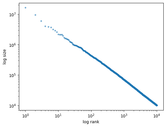
6.2.3. Pareto tails#

In most countries, the cross-sectional distribution of wealth exhibits a Pareto tail (power law).

Let’s see if our model can replicate this stylized fact by running a simulation that generates a cross-section of wealth and generating a suitable rank-size plot.

We will use the function rank_size from quantecon library.

In the limit, data that obeys a power law generates a straight line.

model = create_wealth_model()
key = jax.random.PRNGKey(1234)
ψ_star = update_cross_section_jax_compiled(
        model, ψ_0, num_households, z_sequence, key
)
fig, ax = plt.subplots()

rank_data, size_data = qe.rank_size(ψ_star, c=0.001)
ax.loglog(rank_data, size_data, 'o', markersize=3.0, alpha=0.5)
ax.set_xlabel("log rank")
ax.set_ylabel("log size")

plt.show()

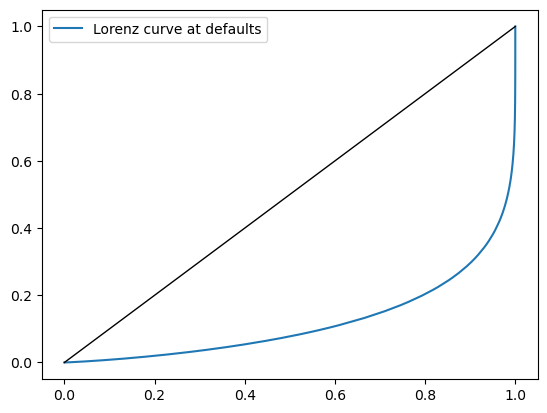
_images/06e2ba95aa9d82f2aa3c395c28b652c57144e9a6ef2c12cbb5dffe2d8ddecd57.png

6.2.4. Lorenz curves and Gini coefficients#

To study the impact of parameters on inequality, we examine Lorenz curves and the Gini coefficients at different parameters.

QuantEcon provides functions to compute Lorenz curves and Gini coefficients that are accelerated using Numba.

Here we provide JAX-based functions that do the same job and are faster for large data sets on parallel hardware.

6.2.4.1. Lorenz curve#

Recall that, for sorted data $w_1, \ldots, w_n$, the Lorenz curve generates data points $(x_i, y_i)_{i=0}^n$ according to

\[ x_0 = y_0 = 0 \qquad \text{and, for $i \geq 1$,} \quad x_i = \frac{i}{n}, \qquad y_i = \frac{\sum_{j \leq i} w_j}{\sum_{j \leq n} w_j} \]

def _lorenz_curve_jax(w, w_size):
    n = w.shape[0]
    w = jnp.sort(w)
    x = jnp.arange(n + 1) / n
    s = jnp.concatenate((jnp.zeros(1), jnp.cumsum(w)))
    y = s / s[n]
    return x, y

lorenz_curve_jax = jax.jit(_lorenz_curve_jax, static_argnums=(1,))

Let’s test

sim_length = 200
num_households = 1_000_000
ψ_0 = jnp.full(num_households, y_mean)  # Initial distribution
z_sequence = generate_aggregate_state_sequence(aggregate_params,
                                               length=sim_length)
z_sequence = jnp.array(z_sequence)

key = jax.random.PRNGKey(1234)
ψ_star = update_cross_section_jax_compiled(
        model, ψ_0, num_households, z_sequence, key
)

%time _ = lorenz_curve_jax(ψ_star, num_households)

CPU times: user 874 ms, sys: 4.02 ms, total: 878 ms
Wall time: 1.35 s

# Now time it without compile time
%time x, y = lorenz_curve_jax(ψ_star, num_households)

CPU times: user 345 µs, sys: 0 ns, total: 345 µs
Wall time: 182 µs

fig, ax = plt.subplots()
ax.plot(x, y, label="Lorenz curve at defaults")
ax.plot(x, x, 'k-', lw=1)
ax.legend()
plt.show()

_images/11447ddec383980fab08ad41b1c206dd77effc19eea8ec9a1511ab7f8f2ff175.png

6.2.4.2. Gini Coefficient#

Recall that, for sorted data $w_1, \ldots, w_n$, the Gini coefficient takes the form

(6.2)#\[ G := \frac {\sum_{i=1}^n \sum_{j = 1}^n |w_j - w_i|} {2n\sum_{i=1}^n w_i}. \]

Here’s a function that computes the Gini coefficient using vectorization.

def _gini_jax(w, w_size):
    w_1 = jnp.reshape(w, (w_size, 1))
    w_2 = jnp.reshape(w, (1, w_size))
    g_sum = jnp.sum(jnp.abs(w_1 - w_2))
    return g_sum / (2 * w_size * jnp.sum(w))

gini_jax = jax.jit(_gini_jax, static_argnums=(1,))

%time gini = gini_jax(ψ_star, num_households).block_until_ready()

CPU times: user 71.8 ms, sys: 4.01 ms, total: 75.8 ms
Wall time: 8.49 s

# Now time it without compilation
%time gini = gini_jax(ψ_star, num_households).block_until_ready()

CPU times: user 2.14 ms, sys: 5 µs, total: 2.14 ms
Wall time: 8.29 s

gini

Array(0.75700235, dtype=float32)

6.3. Exercises#

Exercise 6.1

In this exercise, write an alternative version of gini_jax that uses vmap instead of reshaping and broadcasting.

Test with the same array to see if you can obtain the same output

Solution to Exercise 6.1

Here’s one solution:

@jax.jit
def gini_jax_vmap(w):

    def _inner_sum(x):
        return jnp.sum(jnp.abs(x - w))
    
    inner_sum = jax.vmap(_inner_sum)
    
    full_sum = jnp.sum(inner_sum(w))
    return full_sum / (2 * len(w) * jnp.sum(w))

%time gini = gini_jax_vmap(ψ_star).block_until_ready()

CPU times: user 76.1 ms, sys: 1e+03 ns, total: 76.1 ms
Wall time: 8.41 s

# Now time it without compile time
%time gini = gini_jax_vmap(ψ_star).block_until_ready()

CPU times: user 2.32 ms, sys: 7 µs, total: 2.33 ms
Wall time: 8.38 s

gini

Array(0.75700235, dtype=float32)

Exercise 6.2

In this exercise we investigate how the parameters determining the rate of return on assets and labor income shape inequality.

In doing so we recall that

\[ R_t := 1 + r_t = c_r \exp(z_t) + \exp(\mu_r + \sigma_r \xi_t) \]

while

\[ y_t = c_y \exp(z_t) + \exp(\mu_y + \sigma_y \zeta_t) \]

Investigate how the Lorenz curves and the Gini coefficient associated with the wealth distribution change as return to savings varies.

In particular, plot Lorenz curves for the following three different values of $\mu_r$

μ_r_vals = (0.0, 0.025, 0.05)

Use the following as your initial cross-sectional distribution

num_households = 1_000_000
ψ_0 = jnp.full(num_households, y_mean)  # Initial distribution

Once you have done that, plot the Gini coefficients as well.

Do the outcomes match your intuition?

Solution to Exercise 6.2

Here is one solution

key = jax.random.PRNGKey(1234)
fig, ax = plt.subplots()
gini_vals = []
for μ_r in μ_r_vals:
    model = create_wealth_model(μ_r=μ_r)
    ψ_star = update_cross_section_jax_compiled(
            model, ψ_0, num_households, z_sequence, key
    )
    x, y = lorenz_curve_jax(ψ_star, num_households)
    g = gini_jax(ψ_star, num_households)
    ax.plot(x, y, label=f'$\psi^*$ at $\mu_r = {μ_r:0.2}$')
    gini_vals.append(g)
ax.plot(x, y, label='equality')
ax.legend(loc="upper left")
plt.show()

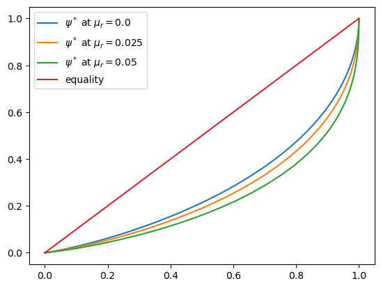
_images/c1a7d29e7f4990a27f98fc140968fadbb9239c2ab1153c474246ea8de560700a.png

The Lorenz curve shifts downwards as returns on financial income rise, indicating a rise in inequality.

Now let’s check the Gini coefficient

fig, ax = plt.subplots()
ax.plot(μ_r_vals, gini_vals, label='Gini coefficient')
ax.set_xlabel("$\mu_r$")
ax.legend()
plt.show()

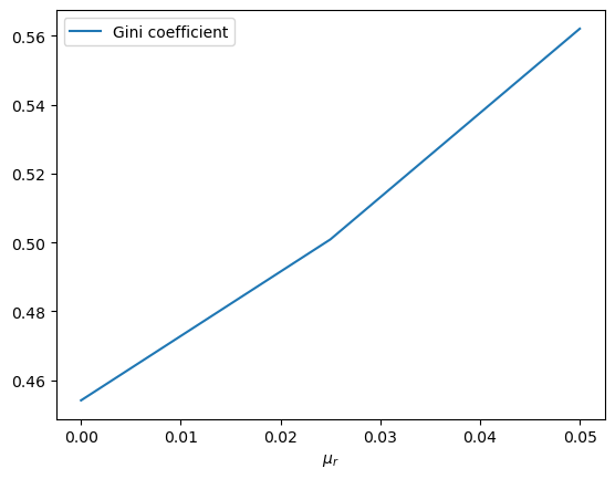
_images/dda75cc5347accfbaea10446e18e764734ec972776bb8be0375ee45c8c87c02d.png

As expected, inequality increases as returns on financial income rise.

Exercise 6.3

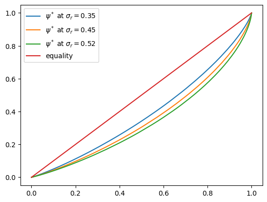
Now investigate what happens when we change the volatility term $\sigma_r$ in financial returns.

Use the same initial condition as before and the sequence

σ_r_vals = (0.35, 0.45, 0.52)

To isolate the role of volatility, set $\mu_r = - \sigma_r^2 / 2$ at each $\sigma_r$.

(This holds the variance of the idiosyncratic term $\exp(\mu_r + \sigma_r \zeta)$ constant.)

Solution to Exercise 6.3

Here’s one solution

key = jax.random.PRNGKey(1234)
fig, ax = plt.subplots()

gini_vals = []
for σ_r in σ_r_vals:
    model = create_wealth_model(σ_r=σ_r, μ_r=(-σ_r**2/2))
    ψ_star = update_cross_section_jax_compiled(
            model, ψ_0, num_households, z_sequence, key
    )
    x, y = lorenz_curve_jax(ψ_star, num_households)
    g = gini_jax(ψ_star, num_households)
    ax.plot(x, y, label=f'$\psi^*$ at $\sigma_r = {σ_r:0.2}$')
    gini_vals.append(g)
ax.plot(x, y, label='equality')
ax.legend(loc="upper left")
plt.show()

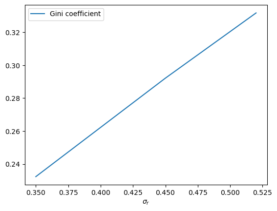
_images/4d7af8079b6a0d4fa1da338925eadba886083d9fdb95741a00ac3242e80baec5.png

fig, ax = plt.subplots()
ax.plot(σ_r_vals, gini_vals, label='Gini coefficient')
ax.set_xlabel("$\sigma_r$")
ax.legend()
plt.show()

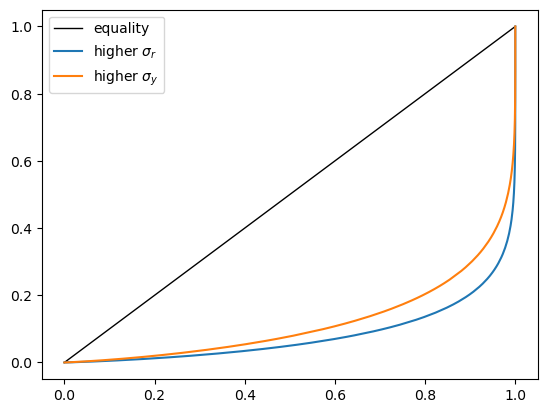
_images/f9d2b4c30540c6040e17308f2b0d237f1c160ed15386a94991b3f36146370a3a.png

Exercise 6.4

In this exercise, examine which has more impact on inequality:

a 5% rise in volatility of the rate of return,
or a 5% rise in volatility of labor income.

Test this by

Shifting $\sigma_r$ up 5% from the baseline and plotting the Lorenz curve
Shifting $\sigma_y$ up 5% from the baseline and plotting the Lorenz curve

Plot both on the same figure and examine the result.

Solution to Exercise 6.4

Here’s one solution.

It shows that increasing volatility in financial income has a greater effect

model = create_wealth_model()
household_params, aggregate_params = model
w_hat, s_0, c_y, μ_y, σ_y, c_r, μ_r, σ_r, y_mean = household_params
σ_r_default = σ_r
σ_y_default = σ_y

ψ_star = update_cross_section_jax_compiled(
            model, ψ_0, num_households, z_sequence, key
)
x_default, y_default = lorenz_curve_jax(ψ_star, num_households)

model = create_wealth_model(σ_r=(1.05 * σ_r_default))
ψ_star = update_cross_section_jax_compiled(
            model, ψ_0, num_households, z_sequence, key
)
x_financial, y_financial = lorenz_curve_jax(ψ_star, num_households)

model = create_wealth_model(σ_y=(1.05 * σ_y_default))
ψ_star = update_cross_section_jax_compiled(
            model, ψ_0, num_households, z_sequence, key
)
x_labor, y_labor = lorenz_curve_jax(ψ_star, num_households)

fig, ax = plt.subplots()    
ax.plot(x_default, x_default, 'k-', lw=1, label='equality')
ax.plot(x_financial, y_financial, label=r'higher $\sigma_r$')
ax.plot(x_labor, y_labor, label=r'higher $\sigma_y$')
ax.legend()
plt.show()

_images/7783c56b5ef40971d685193e14bb51554a7af19ce3bfc477144a68b0e4345d08.png