2. An Introduction to JAX#
GPU
This lecture was built using a machine with access to a GPU — although it will also run without one.
Google Colab has a free tier with GPUs that you can access as follows:
Click on the “play” icon top right
Select Colab
Set the runtime environment to include a GPU
This lecture provides a short introduction to Google JAX.
Let’s see if we have an active GPU:
!nvidia-smi
Thu Jul  9 05:40:44 2026
+-----------------------------------------------------------------------------------------+
| NVIDIA-SMI 580.105.08             Driver Version: 580.105.08     CUDA Version: 13.0     |
+-----------------------------------------+------------------------+----------------------+
| GPU  Name                 Persistence-M | Bus-Id          Disp.A | Volatile Uncorr. ECC |
| Fan  Temp   Perf          Pwr:Usage/Cap |           Memory-Usage | GPU-Util  Compute M. |
|                                         |                        |               MIG M. |
|=========================================+========================+======================|
|   0  Tesla T4                       On  |   00000000:00:1E.0 Off |                    0 |
| N/A   39C    P0             33W /   70W |       0MiB /  15360MiB |      0%      Default |
|                                         |                        |                  N/A |
+-----------------------------------------+------------------------+----------------------+

+-----------------------------------------------------------------------------------------+
| Processes:                                                                              |
|  GPU   GI   CI              PID   Type   Process name                        GPU Memory |
|        ID   ID                                                               Usage      |
|=========================================================================================|
|  No running processes found                                                             |
+-----------------------------------------------------------------------------------------+
2.1. JAX as a NumPy Replacement#
One way to use JAX is as a plug-in NumPy replacement. Let’s look at the similarities and differences.
2.1.1. Similarities#
The following import is standard, replacing import numpy as np:
import jax
import jax.numpy as jnp
Now we can use jnp in place of np for the usual array operations:
a = jnp.asarray((1.0, 3.2, -1.5))
print(a)
[ 1. 3.2 -1.5]
print(jnp.sum(a))
2.6999998
print(jnp.mean(a))
0.9
print(jnp.dot(a, a))
13.490001
However, the array object a is not a NumPy array:
a
Array([ 1. , 3.2, -1.5], dtype=float32)
type(a)
jaxlib._jax.ArrayImpl
Even scalar-valued maps on arrays return JAX arrays.
jnp.sum(a)
Array(2.6999998, dtype=float32)
JAX arrays are also called “device arrays,” where term “device” refers to a hardware accelerator (GPU or TPU).
(In the terminology of GPUs, the “host” is the machine that launches GPU operations, while the “device” is the GPU itself.)
Operations on higher dimensional arrays are also similar to NumPy:
A = jnp.ones((2, 2))
B = jnp.identity(2)
A @ B
Array([[1., 1.],
       [1., 1.]], dtype=float32)
from jax.numpy import linalg
linalg.inv(B) # Inverse of identity is identity
Array([[1., 0.],
       [0., 1.]], dtype=float32)
out = linalg.eigh(B)  # Computes eigenvalues and eigenvectors
out.eigenvalues
Array([0.99999994, 0.99999994], dtype=float32)
out.eigenvectors
Array([[1., 0.],
       [0., 1.]], dtype=float32)
2.1.2. Differences#
One difference between NumPy and JAX is that JAX currently uses 32 bit floats by default.
This is standard for GPU computing and can lead to significant speed gains with small loss of precision.
However, for some calculations precision matters. In these cases 64 bit floats can be enforced via the command
jax.config.update("jax_enable_x64", True)
Let’s check this works:
jnp.ones(3)
Array([1., 1., 1.], dtype=float64)
As a NumPy replacement, a more significant difference is that arrays are treated as immutable.
For example, with NumPy we can write
import numpy as np
a = np.linspace(0, 1, 3)
a
array([0. , 0.5, 1. ])
and then mutate the data in memory:
a[0] = 1
a
array([1. , 0.5, 1. ])
In JAX this fails:
a = jnp.linspace(0, 1, 3)
a
Array([0. , 0.5, 1. ], dtype=float64)
a[0] = 1
---------------------------------------------------------------------------
TypeError                                 Traceback (most recent call last)
Cell In[21], line 1
----> 1 a[0] = 1

File ~/miniconda3/envs/quantecon/lib/python3.13/site-packages/jax/_src/numpy/array_methods.py:975, in _unimplemented_setitem(self, i, x)
    971 def _unimplemented_setitem(self, i, x):
    972   msg = ("JAX arrays are immutable and do not support in-place item assignment."
    973          " Instead of x[idx] = y, use x = x.at[idx].set(y) or another .at[] method:"
    974          " https://docs.jax.dev/en/latest/_autosummary/jax.numpy.ndarray.at.html")
--> 975   raise TypeError(msg)

TypeError: JAX arrays are immutable and do not support in-place item assignment. Instead of x[idx] = y, use x = x.at[idx].set(y) or another .at[] method: https://docs.jax.dev/en/latest/_autosummary/jax.numpy.ndarray.at.html
In line with immutability, JAX does not support inplace operations:
a = np.array((2, 1))
a.sort()
a
array([1, 2])
a = jnp.array((2, 1))
a_new = a.sort()
a, a_new
(Array([2, 1], dtype=int64), Array([1, 2], dtype=int64))
The designers of JAX chose to make arrays immutable because JAX uses a functional programming style. More on this below.
However, JAX provides a functionally pure equivalent of in-place array modification
using the at method.
a = jnp.linspace(0, 1, 3)
id(a)
98175863211280
a
Array([0. , 0.5, 1. ], dtype=float64)
Applying at[0].set(1) returns a new copy of a with the first element set to 1
a = a.at[0].set(1)
a
Array([1. , 0.5, 1. ], dtype=float64)
Inspecting the identifier of a shows that it has been reassigned
id(a)
98175872476848
2.2. Random Numbers#
Random numbers are also a bit different in JAX, relative to NumPy. Typically, in JAX, the state of the random number generator needs to be controlled explicitly.
import jax.random as random
First we produce a key, which seeds the random number generator.
key = random.key(1)
type(key)
jax._src.random.prng.PRNGKeyArray
print(key)
Array((), dtype=key<fry>) overlaying:
[0 1]
Now we can use the key to generate some random numbers:
x = random.normal(key, (3, 3))
x
Array([[-1.18428442, -0.11617041,  0.17269028],
       [ 0.95730718, -0.83295415,  0.69080517],
       [ 0.07545021, -0.7645271 , -0.05064539]], dtype=float64)
If we use the same key again, we initialize at the same seed, so the random numbers are the same:
random.normal(key, (3, 3))
Array([[-1.18428442, -0.11617041,  0.17269028],
       [ 0.95730718, -0.83295415,  0.69080517],
       [ 0.07545021, -0.7645271 , -0.05064539]], dtype=float64)
To produce a (quasi-) independent draw, we can split the existing key.
key, subkey = random.split(key)
random.normal(key, (3, 3))
Array([[ 1.09221959,  0.33192176, -0.90184197],
       [-1.37815779,  0.43052577,  1.6068202 ],
       [ 0.04053753, -0.78732842,  1.75917181]], dtype=float64)
random.normal(subkey, (3, 3))
Array([[ 0.7158846 ,  0.03955972,  0.71127682],
       [-0.40080158, -0.91609481,  0.23713062],
       [ 0.85253995, -0.80972695,  1.79431941]], dtype=float64)
As we will see, the split operation is particularly useful for parallel
computing, where independent sequences or simulations can be given their own
key.
Another option is fold_in, which produces new “independent” keys from a base
key.
The function below produces k (quasi-) independent random n x n matrices using this procedure.
base_key = random.key(42)
def gen_random_matrices(key, n, k):
    matrices = []
    for i in range(k):
        key = random.fold_in(base_key, i)  # generate a fresh key
        matrices.append(random.uniform(key, (n, n)))
    return matrices
matrices = gen_random_matrices(key, 2, 2)
for A in matrices:
    print(A)
[[0.23566993 0.39719189]
 [0.95367373 0.42397776]]
[[0.74211901 0.54715578]
 [0.05988742 0.32206803]]
To get a one-dimensional array of normal random draws, we can either use (len, ) for the shape, as in
random.normal(key, (5, ))
Array([ 1.09221959, 0.33192176, -0.90184197, -1.37815779, 0.43052577], dtype=float64)
or simply use 5 as the shape argument:
random.normal(key, 5)
Array([ 1.09221959, 0.33192176, -0.90184197, -1.37815779, 0.43052577], dtype=float64)
2.3. JIT compilation#
The JAX just-in-time (JIT) compiler accelerates logic within functions by fusing linear algebra operations into a single optimized kernel that the host can launch on the GPU / TPU (or CPU if no accelerator is detected).
2.3.1. A first example#
To see the JIT compiler in action, consider the following function.
def f(x):
    a = 3*x + jnp.sin(x) + jnp.cos(x**2) - jnp.cos(2*x) - x**2 * 0.4 * x**1.5
    return jnp.sum(a)
Let’s build an array to call the function on.
n = 50_000_000
x = jnp.ones(n)
How long does the function take to execute?
%time f(x).block_until_ready()
CPU times: user 448 ms, sys: 11.5 ms, total: 460 ms
Wall time: 639 ms
Array(2.19896006e+08, dtype=float64)
Note
Here, in order to measure actual speed, we use the block_until_ready() method
to hold the interpreter until the results of the computation are returned from
the device. This is necessary because JAX uses asynchronous dispatch, which
allows the Python interpreter to run ahead of GPU computations.
The code doesn’t run as fast as we might hope, given that it’s running on a GPU.
But if we run it a second time it becomes much faster:
%time f(x).block_until_ready()
CPU times: user 3.2 ms, sys: 0 ns, total: 3.2 ms
Wall time: 176 ms
Array(2.19896006e+08, dtype=float64)
This is because the built in functions like jnp.cos are JIT compiled and the
first run includes compile time.
Why would JAX want to JIT-compile built in functions like jnp.cos instead of
just providing pre-compiled versions, like NumPy?
The reason is that the JIT compiler can specialize on the size of the array being used, which is helpful for parallelization.
For example, in running the code above, the JIT compiler produced a version of jnp.cos that is
specialized to floating point arrays of size n = 50_000_000.
We can check this by calling f with a new array of different size.
m = 50_000_001
y = jnp.ones(m)
%time f(y).block_until_ready()
CPU times: user 351 ms, sys: 16.6 ms, total: 368 ms
Wall time: 518 ms
Array(2.19896011e+08, dtype=float64)
Notice that the execution time increases, because now new versions of
the built-ins like jnp.cos are being compiled, specialized to the new array
size.
If we run again, the code is dispatched to the correct compiled version and we get faster execution.
%time f(y).block_until_ready()
CPU times: user 2.97 ms, sys: 187 μs, total: 3.16 ms
Wall time: 108 ms
Array(2.19896011e+08, dtype=float64)
The compiled versions for the previous array size are still available in memory too, and the following call is dispatched to the correct compiled code.
%time f(x).block_until_ready()
CPU times: user 2.27 ms, sys: 860 μs, total: 3.13 ms
Wall time: 123 ms
Array(2.19896006e+08, dtype=float64)
2.3.2. Compiling the outer function#
We can do even better if we manually JIT-compile the outer function.
f_jit = jax.jit(f) # target for JIT compilation
Let’s run once to compile it:
f_jit(x)
Array(2.19896006e+08, dtype=float64)
And now let’s time it.
%time f_jit(x).block_until_ready()
CPU times: user 558 μs, sys: 104 μs, total: 662 μs
Wall time: 69.4 ms
Array(2.19896006e+08, dtype=float64)
Note the speed gain.
This is because the array operations are fused and no intermediate arrays are created.
Incidentally, a more common syntax when targetting a function for the JIT compiler is
@jax.jit
def f(x):
    a = 3*x + jnp.sin(x) + jnp.cos(x**2) - jnp.cos(2*x) - x**2 * 0.4 * x**1.5
    return jnp.sum(a)
2.4. Functional Programming#
From JAX’s documentation:
When walking about the countryside of Italy, the people will not hesitate to tell you that JAX has “una anima di pura programmazione funzionale”.
In other words, JAX assumes a functional programming style.
The major implication is that JAX functions should be pure.
A pure function will always return the same result if invoked with the same inputs.
In particular, a pure function has
no dependence on global variables and
no side effects
JAX will not usually throw errors when compiling impure functions but execution becomes unpredictable.
Here’s an illustration of this fact, using global variables:
a = 1  # global

@jax.jit
def f(x):
    return a + x
x = jnp.ones(2)
f(x)
Array([2., 2.], dtype=float64)
In the code above, the global value a=1 is fused into the jitted function.
Even if we change a, the output of f will not be affected — as long as the same compiled version is called.
a = 42
f(x)
Array([2., 2.], dtype=float64)
Changing the dimension of the input triggers a fresh compilation of the function, at which time the change in the value of a takes effect:
x = jnp.ones(3)
f(x)
Array([43., 43., 43.], dtype=float64)
Moral of the story: write pure functions when using JAX!
2.5. Gradients#
JAX can use automatic differentiation to compute gradients.
This can be extremely useful for optimization and solving nonlinear systems.
We will see significant applications later in this lecture series.
For now, here’s a very simple illustration involving the function
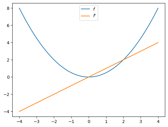
def f(x):
    return (x**2) / 2
Let’s take the derivative:
f_prime = jax.grad(f)
f_prime(10.0)
Array(10., dtype=float64, weak_type=True)
Let’s plot the function and derivative, noting that \(f'(x) = x\).
import matplotlib.pyplot as plt

fig, ax = plt.subplots()
x_grid = jnp.linspace(-4, 4, 200)
ax.plot(x_grid, f(x_grid), label="$f$")
ax.plot(x_grid, [f_prime(x) for x in x_grid], label="$f'$")
ax.legend(loc='upper center')
plt.show()
We defer further exploration of automatic differentiation with JAX until Adventures with Autodiff.
2.6. Writing vectorized code#
Writing fast JAX code requires shifting repetitive tasks from loops to array processing operations, so that the JAX compiler can easily understand the whole operation and generate more efficient machine code.
This procedure is called vectorization or array programming, and will be familiar to anyone who has used NumPy or MATLAB.
In most ways, vectorization is the same in JAX as it is in NumPy.
But there are also some differences, which we highlight here.
As a running example, consider the function
Suppose that we want to evaluate this function on a square grid of \(x\) and \(y\) points and then plot it.
To clarify, here is the slow for loop version.
@jax.jit
def f(x, y):
    return jnp.cos(x**2 + y**2) / (1 + x**2 + y**2)

n = 80
x = jnp.linspace(-2, 2, n)
y = x

z_loops = np.empty((n, n))
%%time
for i in range(n):
    for j in range(n):
        z_loops[i, j] = f(x[i], y[j])
CPU times: user 6.28 s, sys: 2.09 s, total: 8.37 s
Wall time: 5.3 s
Even for this very small grid, the run time is extremely slow.
(Notice that we used a NumPy array for z_loops because we wanted to write to it.)
OK, so how can we do the same operation in vectorized form?
If you are new to vectorization, you might guess that we can simply write
z_bad = f(x, y)
But this gives us the wrong result because JAX doesn’t understand the nested for loop.
z_bad.shape
(80,)
Here is what we actually wanted:
z_loops.shape
(80, 80)
To get the right shape and the correct nested for loop calculation, we can use a meshgrid operation designed for this purpose:
x_mesh, y_mesh = jnp.meshgrid(x, y)
Now we get what we want and the execution time is very fast.
%%time
z_mesh = f(x_mesh, y_mesh).block_until_ready()
CPU times: user 40.4 ms, sys: 3.7 ms, total: 44 ms
Wall time: 76.9 ms
Let’s run again to eliminate compile time.
%%time
z_mesh = f(x_mesh, y_mesh).block_until_ready()
CPU times: user 583 μs, sys: 0 ns, total: 583 μs
Wall time: 312 μs
Let’s confirm that we got the right answer.
jnp.allclose(z_mesh, z_loops)
Array(True, dtype=bool)
Now we can set up a serious grid and run the same calculation (on the larger grid) in a short amount of time.
n = 6000
x = jnp.linspace(-2, 2, n)
y = x
x_mesh, y_mesh = jnp.meshgrid(x, y)
%%time
z_mesh = f(x_mesh, y_mesh).block_until_ready()
CPU times: user 47.4 ms, sys: 4.67 ms, total: 52 ms
Wall time: 126 ms
Let’s run again to get rid of compile time.
%%time
z_mesh = f(x_mesh, y_mesh).block_until_ready()
CPU times: user 543 μs, sys: 131 μs, total: 674 μs
Wall time: 29.1 ms
But there is one problem here: the mesh grids use a lot of memory.
x_mesh.nbytes + y_mesh.nbytes
576000000
By comparison, the flat array x is just
x.nbytes # and y is just a pointer to x
48000
This extra memory usage can be a big problem in actual research calculations.
So let’s try a different approach using jax.vmap
First we vectorize f in y.
f_vec_y = jax.vmap(f, in_axes=(None, 0))
In the line above, (None, 0) indicates that we are vectorizing in the second argument, which is y.
Next, we vectorize in the first argument, which is x.
f_vec = jax.vmap(f_vec_y, in_axes=(0, None))
With this construction, we can now call the function \(f\) on flat (low memory) arrays.
%%time
z_vmap = f_vec(x, y).block_until_ready()
CPU times: user 70.4 ms, sys: 4.57 ms, total: 75 ms
Wall time: 128 ms
We run it again to eliminate compile time.
%%time
z_vmap = f_vec(x, y).block_until_ready()
CPU times: user 1.55 ms, sys: 115 μs, total: 1.66 ms
Wall time: 26.4 ms
The execution time is essentially the same as the mesh operation but we are using much less memory.
And we produce the correct answer:
jnp.allclose(z_vmap, z_mesh)
Array(True, dtype=bool)
2.7. Exercises#
Exercise 2.1
In the Exercise section of a lecture on Numba, we used Monte Carlo to price a European call option.
The code was accelerated by Numba-based multithreading.
Try writing a version of this operation for JAX, using all the same parameters.
If you are running your code on a GPU, you should be able to achieve significantly faster execution.
Solution
Here is one solution:
M = 10_000_000

n, β, K = 20, 0.99, 100
μ, ρ, ν, S0, h0 = 0.0001, 0.1, 0.001, 10, 0

@jax.jit
def compute_call_price_jax(β=β,
                           μ=μ,
                           S0=S0,
                           h0=h0,
                           K=K,
                           n=n,
                           ρ=ρ,
                           ν=ν,
                           M=M,
                           key=jax.random.key(1)):

    s = jnp.full(M, np.log(S0))
    h = jnp.full(M, h0)

    def update(i, loop_state):
        s, h, key = loop_state
        key, subkey = jax.random.split(key)
        Z = jax.random.normal(subkey, (2, M))
        s = s + μ + jnp.exp(h) * Z[0, :]
        h = ρ * h + ν * Z[1, :]
        new_loop_state = s, h, key
        return new_loop_state

    initial_loop_state = s, h, key
    final_loop_state = jax.lax.fori_loop(0, n, update, initial_loop_state)
    s, h, key = final_loop_state

    expectation = jnp.mean(jnp.maximum(jnp.exp(s) - K, 0))

    return β**n * expectation
Note
We use jax.lax.fori_loop instead of a Python for loop.
This allows JAX to compile the loop efficiently without unrolling it,
which significantly reduces compilation time for large arrays.
Let’s run it once to compile it:
%%time
compute_call_price_jax().block_until_ready()
CPU times: user 1.74 s, sys: 45.6 ms, total: 1.79 s
Wall time: 1.56 s
Array(699495.97040563, dtype=float64)
And now let’s time it:
%%time
compute_call_price_jax().block_until_ready()
CPU times: user 3.23 ms, sys: 0 ns, total: 3.23 ms
Wall time: 479 ms
Array(699495.97040563, dtype=float64)