17. Default Risk and Income Fluctuations#
GPU
This lecture was built using a machine with access to a GPU — although it will also run without one.
Google Colab has a free tier with GPUs that you can access as follows:
Click on the “play” icon top right
Select Colab
Set the runtime environment to include a GPU
In addition to JAX and Anaconda, this lecture will need the following libraries:
!pip install quantecon
17.1. Overview#
This lecture computes versions of Arellano’s [Arellano, 2008] model of sovereign default.
The model describes interactions among default risk, output, and an equilibrium interest rate that includes a premium for endogenous default risk.
The decision maker is a government of a small open economy that borrows from risk-neutral foreign creditors.
The foreign lenders must be compensated for default risk.
The government borrows and lends abroad in order to smooth the consumption of its citizens.
The government repays its debt only if it wants to, but declining to pay has adverse consequences.
The interest rate on government debt adjusts in response to the state-dependent default probability chosen by government.
The model yields outcomes that help interpret sovereign default experiences, including
countercyclical interest rates on sovereign debt
countercyclical trade balances
high volatility of consumption relative to output
Notably, long recessions caused by bad draws in the income process increase the government’s incentive to default.
This can lead to
spikes in interest rates
temporary losses of access to international credit markets
large drops in output, consumption, and welfare
large capital outflows during recessions
Such dynamics are consistent with experiences of many countries.
Let’s start with some imports:
import matplotlib.pyplot as plt
import quantecon as qe
import random

import jax
import jax.numpy as jnp
from collections import namedtuple
Let’s check the GPU we are running
!nvidia-smi
Thu Jul  9 05:39:09 2026
+-----------------------------------------------------------------------------------------+
| NVIDIA-SMI 580.105.08             Driver Version: 580.105.08     CUDA Version: 13.0     |
+-----------------------------------------+------------------------+----------------------+
| GPU  Name                 Persistence-M | Bus-Id          Disp.A | Volatile Uncorr. ECC |
| Fan  Temp   Perf          Pwr:Usage/Cap |           Memory-Usage | GPU-Util  Compute M. |
|                                         |                        |               MIG M. |
|=========================================+========================+======================|
|   0  Tesla T4                       On  |   00000000:00:1E.0 Off |                    0 |
| N/A   31C    P8             13W /   70W |       0MiB /  15360MiB |      0%      Default |
|                                         |                        |                  N/A |
+-----------------------------------------+------------------------+----------------------+

+-----------------------------------------------------------------------------------------+
| Processes:                                                                              |
|  GPU   GI   CI              PID   Type   Process name                        GPU Memory |
|        ID   ID                                                               Usage      |
|=========================================================================================|
|  No running processes found                                                             |
+-----------------------------------------------------------------------------------------+
We will use 64 bit floats with JAX in order to increase the precision.
jax.config.update("jax_enable_x64", True)
17.2. Structure#
In this section we describe the main features of the model.
17.2.1. Output, Consumption and Debt#
A small open economy is endowed with an exogenous stochastically fluctuating potential output stream \( \{y_t\} \).
Potential output is realized only in periods in which the government honors its sovereign debt.
The output good can be traded or consumed.
The sequence \( \{y_t\} \) is described by a Markov process with stochastic density kernel \( p(y, y') \).
Households within the country are identical and rank stochastic consumption streams according to
Here
\( 0 < \beta < 1 \) is a time discount factor
\( u \) is an increasing and strictly concave utility function
Consumption sequences enjoyed by households are affected by the government’s decision to borrow or lend internationally.
The government is benevolent in the sense that its aim is to maximize (17.1).
The government is the only domestic actor with access to foreign credit.
Because households are averse to consumption fluctuations, the government will try to smooth consumption by borrowing from (and lending to) foreign creditors.
17.2.2. Asset Markets#
The only credit instrument available to the government is a one-period bond traded in international credit markets.
The bond market has the following features
The bond matures in one period and is not state contingent.
A purchase of a bond with face value \( B' \) is a claim to \( B' \) units of the consumption good next period.
To purchase \( B' \) next period costs \( q B' \) now, or, what is equivalent.
For selling \( -B' \) units of next period goods the seller earns \( - q B' \) of today’s goods.
If \( B' < 0 \), then \( -q B' \) units of the good are received in the current period, for a promise to repay \( -B' \) units next period.
There is an equilibrium price function \( q(B', y) \) that makes \( q \) depend on both \( B' \) and \( y \).
Earnings on the government portfolio are distributed (or, if negative, taxed) lump sum to households.
When the government is not excluded from financial markets, the one-period national budget constraint is
Here and below, a prime denotes a next period value or a claim maturing next period.
To rule out Ponzi schemes, we also require that \( B \geq -Z \) in every period.
\( Z \) is chosen to be sufficiently large that the constraint never binds in equilibrium.
17.2.3. Financial Markets#
Foreign creditors
are risk neutral
know the domestic output stochastic process \( \{y_t\} \) and observe \( y_t, y_{t-1}, \ldots, \) at time \( t \)
can borrow or lend without limit in an international credit market at a constant international interest rate \( r \)
receive full payment if the government chooses to pay
receive zero if the government defaults on its one-period debt due
When a government is expected to default next period with probability \( \delta \), the expected value of a promise to pay one unit of consumption next period is \( 1 - \delta \).
Therefore, the discounted expected value of a promise to pay \( B \) next period is
Next we turn to how the government in effect chooses the default probability \( \delta \).
17.2.4. Government’s Decisions#
At each point in time \( t \), the government chooses between
defaulting
meeting its current obligations and purchasing or selling an optimal quantity of one-period sovereign debt
Defaulting means declining to repay all of its current obligations.
If the government defaults in the current period, then consumption equals current output.
But a sovereign default has two consequences:
Output immediately falls from \( y \) to \( h(y) \), where \( 0 \leq h(y) \leq y \).
It returns to \( y \) only after the country regains access to international credit markets.
The country loses access to foreign credit markets.
17.2.5. Reentering International Credit Market#
While in a state of default, the economy regains access to foreign credit in each subsequent period with probability \( \theta \).
17.3. Equilibrium#
Informally, an equilibrium is a sequence of interest rates on its sovereign debt, a stochastic sequence of government default decisions and an implied flow of household consumption such that
Consumption and assets satisfy the national budget constraint.
The government maximizes household utility taking into account
the resource constraint
the effect of its choices on the price of bonds
consequences of defaulting now for future net output and future borrowing and lending opportunities
The interest rate on the government’s debt includes a risk-premium sufficient to make foreign creditors expect on average to earn the constant risk-free international interest rate.
To express these ideas more precisely, consider first the choices of the government, which
enters a period with initial assets \( B \), or what is the same thing, initial debt to be repaid now of \( -B \)
observes current output \( y \), and
chooses either
to default, or
to pay \( -B \) and set next period’s debt due to \( -B' \)
In a recursive formulation,
state variables for the government comprise the pair \( (B, y) \)
\( v(B, y) \) is the optimum value of the government’s problem when at the beginning of a period it faces the choice of whether to honor or default
\( v_c(B, y) \) is the value of choosing to pay obligations falling due
\( v_d(y) \) is the value of choosing to default
\( v_d(y) \) does not depend on \( B \) because, when access to credit is eventually regained, net foreign assets equal \( 0 \).
Expressed recursively, the value of defaulting is
The value of paying is
The three value functions are linked by
The government chooses to default when
and hence given \( B' \) the probability of default next period is
Given zero profits for foreign creditors in equilibrium, we can combine (17.3) and (17.4) to pin down the bond price function:
17.3.1. Definition of Equilibrium#
An equilibrium is
a pricing function \( q(B',y) \),
a triple of value functions \( (v_c(B, y), v_d(y), v(B,y)) \),
a decision rule telling the government when to default and when to pay as a function of the state \( (B, y) \), and
an asset accumulation rule that, conditional on choosing not to default, maps \( (B,y) \) into \( B' \)
such that
The three Bellman equations for \( (v_c(B, y), v_d(y), v(B,y)) \) are satisfied
Given the price function \( q(B',y) \), the default decision rule and the asset accumulation decision rule attain the optimal value function \( v(B,y) \), and
The price function \( q(B',y) \) satisfies equation (17.5)
17.4. Computation#
Let’s now compute an equilibrium of Arellano’s model.
The equilibrium objects are the value function \( v(B, y) \), the associated default decision rule, and the pricing function \( q(B', y) \).
We’ll use our code to replicate Arellano’s results.
After that we’ll perform some additional simulations.
We use a slightly modified version of the algorithm recommended by Arellano.
The appendix to [Arellano, 2008] recommends value function iteration until convergence, updating the price, and then repeating.
Instead, we update the bond price at every value function iteration step.
The second approach is faster and the two different procedures deliver very similar results.
Here is a more detailed description of our algorithm:
Guess a pair of non-default and default value functions \( v_c \) and \( v_d \).
Using these functions, calculate the value function \( v \), the corresponding default probabilities and the price function \( q \).
At each pair \( (B, y) \),
update the value of defaulting \( v_d(y) \).
update the value of remaining \( v_c(B, y) \).
Check for convergence. If converged, stop – if not, go to step 2.
We use simple discretization on a grid of asset holdings and income levels.
The output process is discretized using a quadrature method due to Tauchen.
As we have in other places, we accelerate our code using Numba.
We define a namedtuple to store parameters, grids and transition probabilities.
ArellanoEconomy = namedtuple('ArellanoEconomy',
    ('β',     # Time discount parameter
    'γ',      # Utility parameter
    'r',      # Lending rate
    'ρ',      # Persistence in the income process
    'η',      # Standard deviation of the income process
    'θ',      # Prob of re-entering financial markets
    'B_size', # Grid size for bonds
    'y_size', # Grid size for income
    'P',      # Markov matrix governing the income process
    'B_grid', # Bond unit grid
    'y_grid', # State values of the income process
    'def_y')) # Default income process
def create_arellano(B_size=251,       # Grid size for bonds
    B_min=-0.45,        # Smallest B value
    B_max=0.45,         # Largest B value
    y_size=51,          # Grid size for income
    β=0.953,            # Time discount parameter
    γ=2.0,              # Utility parameter
    r=0.017,            # Lending rate
    ρ=0.945,            # Persistence in the income process
    η=0.025,            # Standard deviation of the income process
    θ=0.282,            # Prob of re-entering financial markets
    def_y_param=0.969): # Parameter governing income in default

    # Set up grids
    B_grid = jnp.linspace(B_min, B_max, B_size)
    mc = qe.markov.tauchen(y_size, ρ, η)
    y_grid, P = jnp.exp(mc.state_values), mc.P

    # Put grids on the device
    P = jax.device_put(P)

    # Output received while in default, with same shape as y_grid
    def_y = jnp.minimum(def_y_param * jnp.mean(y_grid), y_grid)

    return ArellanoEconomy(β=β, γ=γ, r=r, ρ=ρ, η=η, θ=θ, B_size=B_size,
                            y_size=y_size, P=P,
                            B_grid=B_grid, y_grid=y_grid,
                            def_y=def_y)
Here is the utility function.
@jax.jit
def u(c, γ):
    return c**(1-γ)/(1-γ)
Here is a function to compute the bond price at each state, given \( v_c \) and \( v_d \).
def compute_q(v_c, v_d, params, sizes, arrays):
    """
    Compute the bond price function q(B, y) at each (B, y) pair.  The first
    step is to calculate the default probabilities

        δ(B, y) := Σ_{y'} 1{v_c(B, y') < v_d(y')} P(y, y') dy'

    """

    # Unpack
    β, γ, r, ρ, η, θ = params
    B_size, y_size = sizes
    P, B_grid, y_grid, def_y = arrays

    # Set up arrays with indices [i_B, i_y, i_yp]
    v_d = jnp.reshape(v_d, (1, 1, y_size))
    v_c = jnp.reshape(v_c, (B_size, 1, y_size))
    P = jnp.reshape(P, (1, y_size, y_size))

    # Compute δ[i_B, i_y]
    default_states = v_c < v_d
    delta = jnp.sum(default_states * P, axis=(2,))

    q = (1 - delta ) / (1 + r)
    return q
Next we introduce Bellman operators that updated \( v_d \) and \( v_c \).
def T_d(v_c, v_d, params, sizes, arrays):
    """
    The RHS of the Bellman equation when income is at index y_idx and
    the country has chosen to default.  Returns an update of v_d.
    """
    # Unpack
    β, γ, r, ρ, η, θ = params
    B_size, y_size = sizes
    P, B_grid, y_grid, def_y = arrays


    B0_idx = jnp.searchsorted(B_grid, 1e-10)  # Index at which B is near zero

    current_utility = u(def_y, γ)
    v = jnp.maximum(v_c[B0_idx, :], v_d)
    w = θ * v + (1 - θ) * v_d
    A = jnp.reshape(w, (1, y_size))
    cont_value = jnp.sum(A * P, axis=(1,))

    return current_utility + β * cont_value
def bellman(v_c, v_d, q, params, sizes, arrays):
    """
    The RHS of the Bellman equation when the country is not in a
    defaulted state on their debt.  That is,

        bellman(B, y) =
            u(y - q(B', y) B' + B) + β Σ_{y'} v(B', y') P(y, y')

    If consumption is not positive then returns -np.inf
    """
    # Unpack
    β, γ, r, ρ, η, θ = params
    B_size, y_size = sizes
    P, B_grid, y_grid, def_y = arrays

    # Set up c[i_B, i_y, i_Bp]
    y_idx = jnp.reshape(jnp.arange(y_size), (1, y_size, 1))
    B_idx = jnp.reshape(jnp.arange(B_size), (B_size, 1, 1))
    Bp_idx = jnp.reshape(jnp.arange(B_size), (1, 1, B_size))
    c = y_grid[y_idx] - q[Bp_idx, y_idx] * B_grid[Bp_idx] + B_grid[B_idx]

    # Set up v[i_B, i_y, i_Bp, i_yp] and P[i_B, i_y, i_Bp, i_yp]
    v_d = jnp.reshape(v_d, (1, 1, 1, y_size))
    v_c = jnp.reshape(v_c, (1, 1, B_size, y_size))
    v = jnp.maximum(v_c, v_d)
    P = jnp.reshape(P, (1, y_size, 1, y_size))
    # Sum over i_yp
    continuation_value = jnp.sum(v * P, axis=(3,))

    # Return new_v_c[i_B, i_y, i_Bp]
    val = jnp.where(c > 0, u(c, γ) + β * continuation_value, -jnp.inf)
    return val
def T_c(v_c, v_d, q, params, sizes, arrays):
    vals = bellman(v_c, v_d, q, params, sizes, arrays)
    return jnp.max(vals, axis=2)
def get_greedy(v_c, v_d, q, params, sizes, arrays):
    vals = bellman(v_c, v_d, q, params, sizes, arrays)
    return jnp.argmax(vals, axis=2)
Let’s make JIT-compiled versions of these functions, with the sizes of the arrays declared as static (compile-time constants) in order to help the compiler.
compute_q = jax.jit(compute_q, static_argnums=(3,))
T_d = jax.jit(T_d, static_argnums=(3,))
bellman = jax.jit(bellman, static_argnums=(4,))
T_c = jax.jit(T_c, static_argnums=(4,))
get_greedy = jax.jit(get_greedy, static_argnums=(4,))
Here is a function that calls these operators in the right sequence.
def update_values_and_prices(v_c, v_d, params, sizes, arrays):

    q = compute_q(v_c, v_d, params, sizes, arrays)
    new_v_d = T_d(v_c, v_d, params, sizes, arrays)
    new_v_c = T_c(v_c, v_d, q, params, sizes, arrays)

    return new_v_c, new_v_d
We can now write a function that will use an instance of ArellanoEconomy and
the functions defined above to compute the solution to our model.
One of the jobs of this function is to take an instance of
ArellanoEconomy, which is hard for the JIT compiler to handle, and strip it
down to more basic objects, which are then passed out to jitted functions.
def solve(model, tol=1e-8, max_iter=10_000):
    """
    Given an instance of `ArellanoEconomy`, this function computes the optimal
    policy and value functions.
    """
    # Unpack

    β, γ, r, ρ, η, θ, B_size, y_size, P, B_grid, y_grid, def_y = model

    params = β, γ, r, ρ, η, θ
    sizes = B_size, y_size
    arrays = P, B_grid, y_grid, def_y

    β, γ, r, ρ, η, θ, B_size, y_size, P, B_grid, y_grid, def_y = model

    params = β, γ, r, ρ, η, θ
    sizes = B_size, y_size
    arrays = P, B_grid, y_grid, def_y

    # Initial conditions for v_c and v_d
    v_c = jnp.zeros((B_size, y_size))
    v_d = jnp.zeros((y_size,))

    current_iter = 0
    error = tol + 1
    while (current_iter < max_iter) and (error > tol):
        if current_iter % 100 == 0:
            print(f"Entering iteration {current_iter} with error {error}.")
        new_v_c, new_v_d = update_values_and_prices(v_c, v_d, params,
                                                    sizes, arrays)
        error = jnp.max(jnp.abs(new_v_c - v_c)) + jnp.max(jnp.abs(new_v_d - v_d))
        v_c, v_d = new_v_c, new_v_d
        current_iter += 1

    print(f"Terminating at iteration {current_iter}.")

    q = compute_q(v_c, v_d, params, sizes, arrays)
    B_star = get_greedy(v_c, v_d, q, params, sizes, arrays)
    return v_c, v_d, q, B_star
Let’s try solving the model.
ae = create_arellano()
%%time
v_c, v_d, q, B_star = solve(ae)
Entering iteration 0 with error 1.00000001.
Entering iteration 100 with error 0.017499341639204857.
Entering iteration 200 with error 0.00014189363558969603.
Entering iteration 300 with error 1.151467966309383e-06.
Terminating at iteration 399.
CPU times: user 1.55 s, sys: 226 ms, total: 1.77 s
Wall time: 2.98 s
We run it again to get rid of compile time.
%%time
v_c, v_d, q, B_star = solve(ae)
Entering iteration 0 with error 1.00000001.
Entering iteration 100 with error 0.017499341639204857.
Entering iteration 200 with error 0.00014189363558969603.
Entering iteration 300 with error 1.151467966309383e-06.
Terminating at iteration 399.
CPU times: user 647 ms, sys: 181 ms, total: 828 ms
Wall time: 1.59 s
Finally, we write a function that will allow us to simulate the economy once we have the policy functions
def simulate(model, T, v_c, v_d, q, B_star, key):
    """
    Simulates the Arellano 2008 model of sovereign debt

    Here `model` is an instance of `ArellanoEconomy` and `T` is the length of
    the simulation.  Endogenous objects `v_c`, `v_d`, `q` and `B_star` are
    assumed to come from a solution to `model`.

    """
    # Unpack elements of the model
    B_size, y_size = model.B_size, model.y_size
    B_grid, y_grid, P = model.B_grid, model.y_grid, model.P

    B0_idx = jnp.searchsorted(B_grid, 1e-10)  # Index at which B is near zero

    # Set initial conditions
    y_idx = y_size // 2
    B_idx = B0_idx
    in_default = False

    # Create Markov chain and simulate income process
    mc = qe.MarkovChain(P, y_grid)
    y_sim_indices = mc.simulate_indices(T+1, init=y_idx)

    # Allocate memory for outputs
    y_sim = jnp.empty(T)
    y_a_sim = jnp.empty(T)
    B_sim = jnp.empty(T)
    q_sim = jnp.empty(T)
    d_sim = jnp.empty(T, dtype=int)

    # Perform simulation
    t = 0
    while t < T:

        # Update y_sim and B_sim
        y_sim = y_sim.at[t].set(y_grid[y_idx])
        B_sim = B_sim.at[t].set(B_grid[B_idx])

        # if in default:
        if v_c[B_idx, y_idx] < v_d[y_idx] or in_default:
            # Update y_a_sim
            y_a_sim = y_a_sim.at[t].set(model.def_y[y_idx])
            d_sim = d_sim.at[t].set(1)
            Bp_idx = B0_idx
            # Re-enter financial markets next period with prob θ
            # in_default = False if jnp.random.rand() < model.θ else True
            in_default = False if random.uniform(key) < model.θ else True
            key, _ = random.split(key)  # Update the random key
        else:
            # Update y_a_sim
            y_a_sim = y_a_sim.at[t].set(y_sim[t])
            d_sim = d_sim.at[t].set(0)
            Bp_idx = B_star[B_idx, y_idx]

        q_sim = q_sim.at[t].set(q[Bp_idx, y_idx])

        # Update time and indices
        t += 1
        y_idx = y_sim_indices[t]
        B_idx = Bp_idx

    return y_sim, y_a_sim, B_sim, q_sim, d_sim
17.5. Results#
Let’s start by trying to replicate the results obtained in [Arellano, 2008].
In what follows, all results are computed using parameter values of ArellanoEconomy created by create_arellano.
For example, r=0.017 matches the average quarterly rate on a 5 year US treasury over the period 1983–2001.
Details on how to compute the figures are reported as solutions to the exercises.
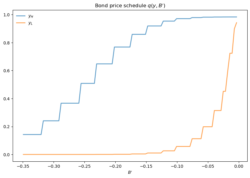
The first figure shows the bond price schedule and replicates Figure 3 of [Arellano, 2008], where \( y_L \) and \( Y_H \) are particular below average and above average values of output \( y \).
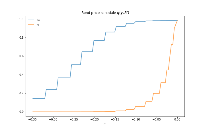
\( y_L \) is 5% below the mean of the \( y \) grid values
\( y_H \) is 5% above the mean of the \( y \) grid values
The grid used to compute this figure was relatively fine (y_size, B_size = 51, 251),
which explains the minor differences between this and Arrelano’s figure.
The figure shows that
Higher levels of debt (larger \( -B' \)) induce larger discounts on the face value, which correspond to higher interest rates.
Lower income also causes more discounting, as foreign creditors anticipate greater likelihood of default.
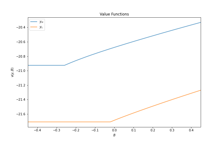
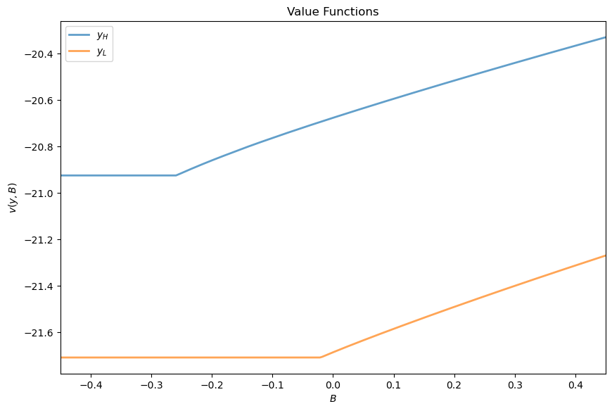
The next figure plots value functions and replicates the right hand panel of Figure 4 of [Arellano, 2008].
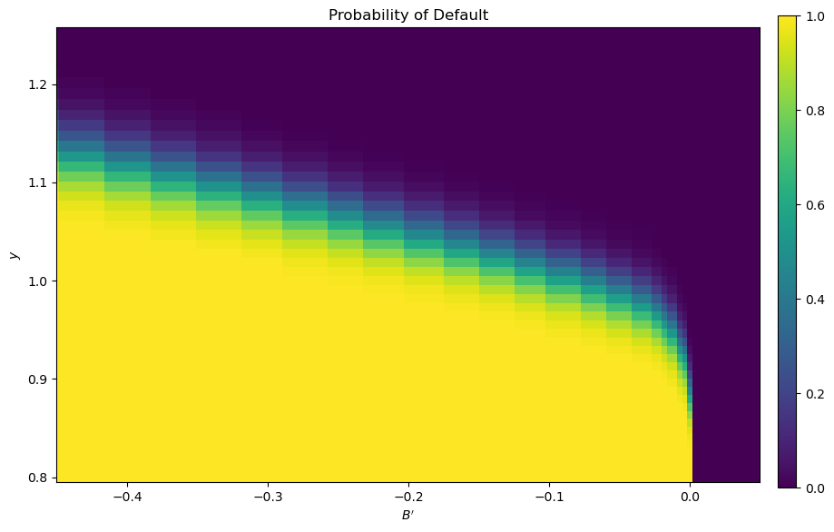
We can use the results of the computation to study the default probability \( \delta(B', y) \) defined in (17.4).
The next plot shows these default probabilities over \( (B', y) \) as a heat map.
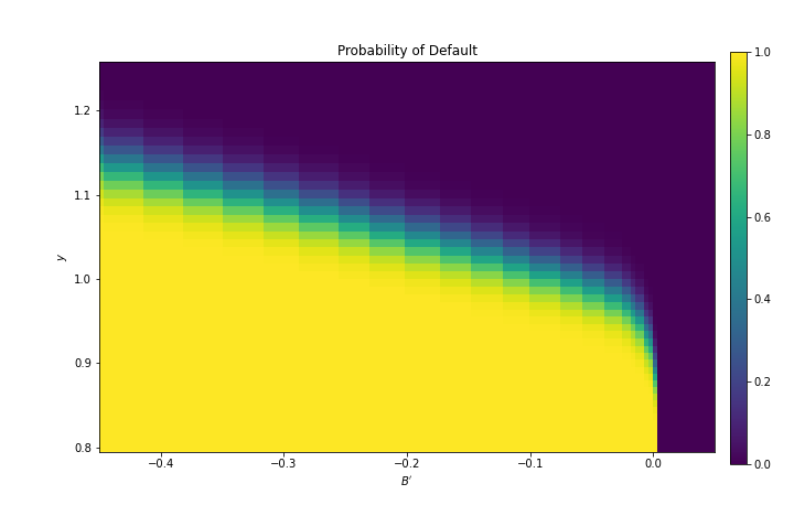
As anticipated, the probability that the government chooses to default in the following period increases with indebtedness and falls with income.
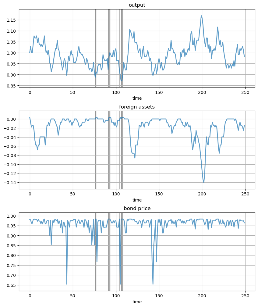
Next let’s run a time series simulation of \( \{y_t\} \), \( \{B_t\} \) and \( q(B_{t+1}, y_t) \).
The grey vertical bars correspond to periods when the economy is excluded from financial markets because of a past default.
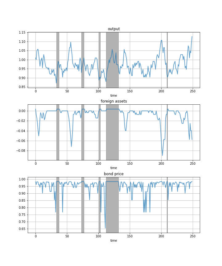
One notable feature of the simulated data is the nonlinear response of interest rates.
Periods of relative stability are followed by sharp spikes in the discount rate on government debt.
17.6. Exercises#
Exercise 17.1
To the extent that you can, replicate the figures shown above
Use the parameter values listed as defaults in
ArellanoEconomycreated bycreate_arellano.The time series will of course vary depending on the shock draws.
Solution
Compute the value function, policy and equilibrium prices
ae = create_arellano()
v_c, v_d, q, B_star = solve(ae)
Entering iteration 0 with error 1.00000001.
Entering iteration 100 with error 0.017499341639204857.
Entering iteration 200 with error 0.00014189363558969603.
Entering iteration 300 with error 1.151467966309383e-06.
Terminating at iteration 399.
Compute the bond price schedule as seen in figure 3 of [Arellano, 2008]
# Unpack some useful names
B_grid, y_grid, P = ae.B_grid, ae.y_grid, ae.P
B_size, y_size = ae.B_size, ae.y_size
r = ae.r

# Create "Y High" and "Y Low" values as 5% devs from mean
high, low = jnp.mean(y_grid) * 1.05, jnp.mean(y_grid) * .95
iy_high, iy_low = (jnp.searchsorted(y_grid, x) for x in (high, low))

fig, ax = plt.subplots(figsize=(10, 6.5))
ax.set_title("Bond price schedule $q(y, B')$")

# Extract a suitable plot grid
x = []
q_low = []
q_high = []
for i, B in enumerate(B_grid):
    if -0.35 <= B <= 0:  # To match fig 3 of Arellano (2008)
        x.append(B)
        q_low.append(q[i, iy_low])
        q_high.append(q[i, iy_high])
ax.plot(x, q_high, label="$y_H$", lw=2, alpha=0.7)
ax.plot(x, q_low, label="$y_L$", lw=2, alpha=0.7)
ax.set_xlabel("$B'$")
ax.legend(loc='upper left', frameon=False)
plt.show()
Draw a plot of the value functions
v = jnp.maximum(v_c, jnp.reshape(v_d, (1, y_size)))

fig, ax = plt.subplots(figsize=(10, 6.5))
ax.set_title("Value Functions")
ax.plot(B_grid, v[:, iy_high], label="$y_H$", lw=2, alpha=0.7)
ax.plot(B_grid, v[:, iy_low], label="$y_L$", lw=2, alpha=0.7)
ax.legend(loc='upper left')
ax.set(xlabel="$B$", ylabel="$v(y, B)$")
ax.set_xlim(min(B_grid), max(B_grid))
plt.show()
Draw a heat map for default probability
# Set up arrays with indices [i_B, i_y, i_yp]
shaped_v_d = jnp.reshape(v_d, (1, 1, y_size))
shaped_v_c = jnp.reshape(v_c, (B_size, 1, y_size))
shaped_P = jnp.reshape(P, (1, y_size, y_size))

# Compute delta[i_B, i_y]
default_states = 1.0 * (shaped_v_c < shaped_v_d)
delta = jnp.sum(default_states * shaped_P, axis=(2,))

# Create figure
fig, ax = plt.subplots(figsize=(10, 6.5))
hm = ax.pcolormesh(B_grid, y_grid, delta.T)
cax = fig.add_axes([.92, .1, .02, .8])
fig.colorbar(hm, cax=cax)
ax.axis([B_grid.min(), 0.05, y_grid.min(), y_grid.max()])
ax.set(xlabel="$B'$", ylabel="$y$", title="Probability of Default")
plt.show()
Plot a time series of major variables simulated from the model
import jax.random as random
T = 250
key = random.key(42)
y_sim, y_a_sim, B_sim, q_sim, d_sim = simulate(ae, T, v_c, v_d, q, B_star, key)

# T = 250
# jnp.random.seed(42)
# y_sim, y_a_sim, B_sim, q_sim, d_sim = simulate(ae, T, v_c, v_d, q, B_star)
# Pick up default start and end dates
start_end_pairs = []
i = 0
while i < len(d_sim):
    if d_sim[i] == 0:
        i += 1
    else:
        # If we get to here we're in default
        start_default = i
        while i < len(d_sim) and d_sim[i] == 1:
            i += 1
        end_default = i - 1
        start_end_pairs.append((start_default, end_default))

plot_series = (y_sim, B_sim, q_sim)
titles = 'output', 'foreign assets', 'bond price'

fig, axes = plt.subplots(len(plot_series), 1, figsize=(10, 12))
fig.subplots_adjust(hspace=0.3)

for ax, series, title in zip(axes, plot_series, titles):
    # Determine suitable y limits
    s_max, s_min = max(series), min(series)
    s_range = s_max - s_min
    y_max = s_max + s_range * 0.1
    y_min = s_min - s_range * 0.1
    ax.set_ylim(y_min, y_max)
    for pair in start_end_pairs:
        ax.fill_between(pair, (y_min, y_min), (y_max, y_max),
                        color='k', alpha=0.3)
    ax.grid()
    ax.plot(range(T), series, lw=2, alpha=0.7)
    ax.set(title=title, xlabel="time")

plt.show()