10. Optimal Savings I: Value Function Iteration#

GPU

This lecture was built using a machine with JAX installed and access to a GPU.

To run this lecture on Google Colab, click on the “play” icon top right, select Colab, and set the runtime environment to include a GPU.

To run this lecture on your own machine, you need to install Google JAX.

In addition to JAX and Anaconda, this lecture will need the following libraries:

!pip install quantecon

We will use the following imports:

import quantecon as qe
import numpy as np
import jax
import jax.numpy as jnp
import matplotlib.pyplot as plt
from collections import namedtuple
from time import time

Let’s check the GPU we are running

!nvidia-smi

Thu Jun 13 04:28:32 2024       
+---------------------------------------------------------------------------------------+
| NVIDIA-SMI 535.54.03              Driver Version: 535.54.03    CUDA Version: 12.5     |
|-----------------------------------------+----------------------+----------------------+
| GPU  Name                 Persistence-M | Bus-Id        Disp.A | Volatile Uncorr. ECC |
| Fan  Temp   Perf          Pwr:Usage/Cap |         Memory-Usage | GPU-Util  Compute M. |
|                                         |                      |               MIG M. |
|=========================================+======================+======================|
|   0  Tesla T4                       On  | 00000001:00:00.0 Off |                  Off |
| N/A   49C    P8               9W /  70W |      2MiB / 16384MiB |      0%      Default |
|                                         |                      |                  N/A |
+-----------------------------------------+----------------------+----------------------+
                                                                                         
+---------------------------------------------------------------------------------------+
| Processes:                                                                            |
|  GPU   GI   CI        PID   Type   Process name                            GPU Memory |
|        ID   ID                                                             Usage      |
|=======================================================================================|
|  No running processes found                                                           |
+---------------------------------------------------------------------------------------+

We’ll use 64 bit floats to gain extra precision.

jax.config.update("jax_enable_x64", True)

10.1. Overview#

We consider an optimal savings problem with CRRA utility and budget constraint

\[ W_{t+1} + C_t \leq R W_t + Y_t \]

where

\(C_t\) is consumption and \(C_t \geq 0\),
\(W_t\) is wealth and \(W_t \geq 0\),
\(R > 0\) is a gross rate of return, and
\((Y_t)\) is labor income.

We assume below that labor income is a discretized AR(1) process.

The Bellman equation is

\[ v(w) = \max_{0 \leq w' \leq Rw + y} \left\{ u(Rw + y - w') + β \sum_{y'} v(w', y') Q(y, y') \right\} \]

where

\[ u(c) = \frac{c^{1-\gamma}}{1-\gamma} \]

In the code we use the function

\[ B((w, y), w', v) = u(Rw + y - w') + β \sum_{y'} v(w', y') Q(y, y'). \]

the encapsulate the right hand side of the Bellman equation.

10.2. Starting with NumPy#

Let’s start with a standard NumPy version running on the CPU.

Starting with this traditional approach will allow us to record the speed gain associated with switching to JAX.

(NumPy operations are similar to MATLAB operations, so this also serves as a rough comparison with MATLAB.)

10.2.1. Functions and operators#

The following function contains default parameters and returns tuples that contain the key computational components of the model.

def create_consumption_model(R=1.01,                    # Gross interest rate
                             β=0.98,                    # Discount factor
                             γ=2,                       # CRRA parameter
                             w_min=0.01,                # Min wealth
                             w_max=5.0,                 # Max wealth
                             w_size=150,                # Grid side
                             ρ=0.9, ν=0.1, y_size=100): # Income parameters
    """
    A function that takes in parameters and returns parameters and grids 
    for the optimal savings problem.
    """
    # Build grids and transition probabilities
    w_grid = np.linspace(w_min, w_max, w_size)
    mc = qe.tauchen(n=y_size, rho=ρ, sigma=ν)
    y_grid, Q = np.exp(mc.state_values), mc.P
    # Pack and return
    params = β, R, γ
    sizes = w_size, y_size
    arrays = w_grid, y_grid, Q
    return params, sizes, arrays

(The function returns sizes of arrays because we use them later to help compile functions in JAX.)

To produce efficient NumPy code, we will use a vectorized approach.

The first step is to create the right hand side of the Bellman equation as a multi-dimensional array with dimensions over all states and controls.

def B(v, params, sizes, arrays):
    """
    A vectorized version of the right-hand side of the Bellman equation
    (before maximization), which is a 3D array representing

        B(w, y, w′) = u(Rw + y - w′) + β Σ_y′ v(w′, y′) Q(y, y′)

    for all (w, y, w′).
    """

    # Unpack
    β, R, γ = params
    w_size, y_size = sizes
    w_grid, y_grid, Q = arrays

    # Compute current rewards r(w, y, wp) as array r[i, j, ip]
    w  = np.reshape(w_grid, (w_size, 1, 1))    # w[i]   ->  w[i, j, ip]
    y  = np.reshape(y_grid, (1, y_size, 1))    # z[j]   ->  z[i, j, ip]
    wp = np.reshape(w_grid, (1, 1, w_size))    # wp[ip] -> wp[i, j, ip]
    c = R * w + y - wp

    # Calculate continuation rewards at all combinations of (w, y, wp)
    v = np.reshape(v, (1, 1, w_size, y_size))  # v[ip, jp] -> v[i, j, ip, jp]
    Q = np.reshape(Q, (1, y_size, 1, y_size))  # Q[j, jp]  -> Q[i, j, ip, jp]
    EV = np.sum(v * Q, axis=3)                 # sum over last index jp

    # Compute the right-hand side of the Bellman equation
    return np.where(c > 0, c**(1-γ)/(1-γ) + β * EV, -np.inf)

Here are two functions we need for value function iteration.

The first is the Bellman operator.

The second computes a \(v\)-greedy policy given \(v\) (i.e., the policy that maximizes the right-hand side of the Bellman equation.)

def T(v, params, sizes, arrays):
    "The Bellman operator."
    return np.max(B(v, params, sizes, arrays), axis=2)

def get_greedy(v, params, sizes, arrays):
    "Computes a v-greedy policy, returned as a set of indices."
    return np.argmax(B(v, params, sizes, arrays), axis=2)

10.2.2. Value function iteration#

Here’s a routine that performs value function iteration.

def value_function_iteration(model, max_iter=10_000, tol=1e-5):
    params, sizes, arrays = model
    v = np.zeros(sizes)
    i, error = 0, tol + 1
    while error > tol and i < max_iter:
        v_new = T(v, params, sizes, arrays)
        error = np.max(np.abs(v_new - v))
        i += 1
        v = v_new
    return v, get_greedy(v, params, sizes, arrays)

Now we create an instance, unpack it, and test how long it takes to solve the model.

model = create_consumption_model()
# Unpack
params, sizes, arrays = model
β, R, γ = params
w_size, y_size = sizes
w_grid, y_grid, Q = arrays

print("Starting VFI.")
start = time()
v_star, σ_star = value_function_iteration(model)
numpy_with_compile = time() - start
print(f"VFI completed in {numpy_with_compile} seconds.")

Starting VFI.

VFI completed in 11.808090209960938 seconds.

Let’s run it again to eliminate compile time.

start = time()
v_star, σ_star = value_function_iteration(model)
numpy_without_compile = time() - start
print(f"VFI completed in {numpy_without_compile} seconds.")

VFI completed in 11.82644271850586 seconds.

Here’s a plot of the policy function.

fig, ax = plt.subplots()
ax.plot(w_grid, w_grid, "k--", label="45")
ax.plot(w_grid, w_grid[σ_star[:, 1]], label="$\\sigma^*(\cdot, y_1)$")
ax.plot(w_grid, w_grid[σ_star[:, -1]], label="$\\sigma^*(\cdot, y_N)$")
ax.legend()
plt.show()

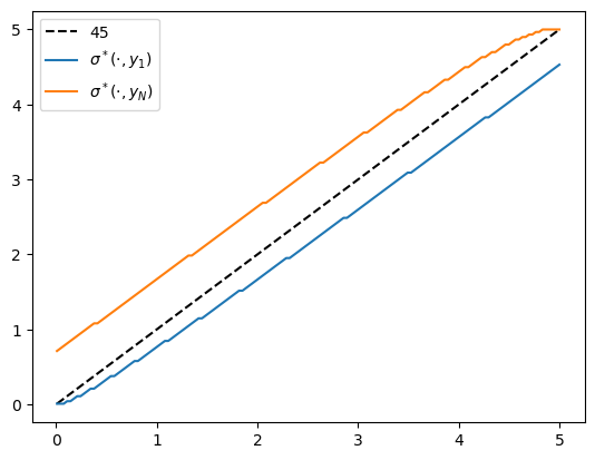
_images/75cfbd4c96fe584c8f8987f37e22c7e34130b96b75afddceebea474b34c3884e.png — Fig. 10.1 Policy function#

10.3. Switching to JAX#

To switch over to JAX, we change np to jnp throughout and add some jax.jit requests.

10.3.1. Functions and operators#

We redefine create_consumption_model to produce JAX arrays.

def create_consumption_model(R=1.01,                    # Gross interest rate
                             β=0.98,                    # Discount factor
                             γ=2,                       # CRRA parameter
                             w_min=0.01,                # Min wealth
                             w_max=5.0,                 # Max wealth
                             w_size=150,                # Grid side
                             ρ=0.9, ν=0.1, y_size=100): # Income parameters
    """
    A function that takes in parameters and returns parameters and grids 
    for the optimal savings problem.
    """
    w_grid = jnp.linspace(w_min, w_max, w_size)
    mc = qe.tauchen(n=y_size, rho=ρ, sigma=ν)
    y_grid, Q = jnp.exp(mc.state_values), jax.device_put(mc.P)
    sizes = w_size, y_size
    return (β, R, γ), sizes, (w_grid, y_grid, Q)

The right hand side of the Bellman equation is the same as the NumPy version after switching np to jnp.

def B(v, params, sizes, arrays):
    """
    A vectorized version of the right-hand side of the Bellman equation
    (before maximization), which is a 3D array representing

        B(w, y, w′) = u(Rw + y - w′) + β Σ_y′ v(w′, y′) Q(y, y′)

    for all (w, y, w′).
    """

    # Unpack
    β, R, γ = params
    w_size, y_size = sizes
    w_grid, y_grid, Q = arrays

    # Compute current rewards r(w, y, wp) as array r[i, j, ip]
    w  = jnp.reshape(w_grid, (w_size, 1, 1))    # w[i]   ->  w[i, j, ip]
    y  = jnp.reshape(y_grid, (1, y_size, 1))    # z[j]   ->  z[i, j, ip]
    wp = jnp.reshape(w_grid, (1, 1, w_size))    # wp[ip] -> wp[i, j, ip]
    c = R * w + y - wp

    # Calculate continuation rewards at all combinations of (w, y, wp)
    v = jnp.reshape(v, (1, 1, w_size, y_size))  # v[ip, jp] -> v[i, j, ip, jp]
    Q = jnp.reshape(Q, (1, y_size, 1, y_size))  # Q[j, jp]  -> Q[i, j, ip, jp]
    EV = jnp.sum(v * Q, axis=3)                 # sum over last index jp

    # Compute the right-hand side of the Bellman equation
    return jnp.where(c > 0, c**(1-γ)/(1-γ) + β * EV, -jnp.inf)

Some readers might be concerned that we are creating high dimensional arrays, leading to inefficiency.

Could they be avoided by more careful vectorization?

In fact this is not necessary: this function will be JIT-compiled by JAX, and the JIT compiler will optimize compiled code to minimize memory use.

B = jax.jit(B, static_argnums=(2,))

In the call above, we indicate to the compiler that sizes is static, so the compiler can parallelize optimally while taking array sizes as fixed.

The Bellman operator \(T\) can be implemented by

def T(v, params, sizes, arrays):
    "The Bellman operator."
    return jnp.max(B(v, params, sizes, arrays), axis=2)

T = jax.jit(T, static_argnums=(2,))

The next function computes a \(v\)-greedy policy given \(v\) (i.e., the policy that maximizes the right-hand side of the Bellman equation.)

def get_greedy(v, params, sizes, arrays):
    "Computes a v-greedy policy, returned as a set of indices."
    return jnp.argmax(B(v, params, sizes, arrays), axis=2)

get_greedy = jax.jit(get_greedy, static_argnums=(2,))

10.3.2. Successive approximation#

Now we define a solver that implements VFI.

We could use the one we built for NumPy above, after changing np to jnp.

Alternatively, we can push a bit harder and write a compiled version using jax.lax.while_loop.

This will give us just a bit more speed.

The first step is to write a compiled successive approximation routine that performs fixed point iteration on some given function T.

def successive_approx_jax(T,                     # Operator (callable)
                          x_0,                   # Initial condition                
                          tolerance=1e-6,        # Error tolerance
                          max_iter=10_000):      # Max iteration bound
    def body_fun(k_x_err):
        k, x, error = k_x_err
        x_new = T(x)
        error = jnp.max(jnp.abs(x_new - x))
        return k + 1, x_new, error

    def cond_fun(k_x_err):
        k, x, error = k_x_err
        return jnp.logical_and(error > tolerance, k < max_iter)

    k, x, error = jax.lax.while_loop(cond_fun, body_fun, 
                                    (1, x_0, tolerance + 1))
    return x

successive_approx_jax = \
    jax.jit(successive_approx_jax, static_argnums=(0,))

Our value function iteration routine calls successive_approx_jax while passing in the Bellman operator.

def value_function_iteration(model, tol=1e-5):
    params, sizes, arrays = model
    vz = jnp.zeros(sizes)
    _T = lambda v: T(v, params, sizes, arrays)
    v_star = successive_approx_jax(_T, vz, tolerance=tol)
    return v_star, get_greedy(v_star, params, sizes, arrays)

10.3.3. Timing#

Let’s create an instance and unpack it.

model = create_consumption_model()
# Unpack
params, sizes, arrays = model
β, R, γ = params
w_size, y_size = sizes
w_grid, y_grid, Q = arrays

Let’s see how long it takes to solve this model.

print("Starting VFI using vectorization.")
start = time()
v_star_jax, σ_star_jax = value_function_iteration(model)
jax_with_compile = time() - start
print(f"VFI completed in {jax_with_compile} seconds.")

Starting VFI using vectorization.

VFI completed in 0.6622564792633057 seconds.

Let’s run it again to eliminate compile time.

start = time()
v_star_jax, σ_star_jax = value_function_iteration(model)
jax_without_compile = time() - start
print(f"VFI completed in {jax_without_compile} seconds.")

VFI completed in 0.31258082389831543 seconds.

The relative speed gain is

print(f"Relative speed gain = {numpy_without_compile / jax_without_compile}")

Relative speed gain = 37.8348312318515

This is an impressive speed up and in fact we can do better still by switching to alternative algorithms that are better suited to parallelization.

These algorithms are discussed in a separate lecture.

10.4. Switching to vmap#

Before we discuss alternative algorithms, let’s take another look at value function iteration.

For this simple optimal savings problem, direct vectorization is relatively easy.

In particular, it’s straightforward to express the right hand side of the Bellman equation as an array that stores evaluations of the function at every state and control.

For more complex models direct vectorization can be much harder.

For this reason, it helps to have another approach to fast JAX implementations up our sleeves.

Here’s a version that

writes the right hand side of the Bellman operator as a function of individual states and controls, and
applies jax.vmap on the outside to achieve a parallelized solution.

First let’s rewrite B

def B(v, params, arrays, i, j, ip):
    """
    The right-hand side of the Bellman equation before maximization, which takes
    the form

        B(w, y, w′) = u(Rw + y - w′) + β Σ_y′ v(w′, y′) Q(y, y′)

    The indices are (i, j, ip) -> (w, y, w′).
    """
    β, R, γ = params
    w_grid, y_grid, Q = arrays
    w, y, wp  = w_grid[i], y_grid[j], w_grid[ip]
    c = R * w + y - wp
    EV = jnp.sum(v[ip, :] * Q[j, :]) 
    return jnp.where(c > 0, c**(1-γ)/(1-γ) + β * EV, -jnp.inf)

Now we successively apply vmap to simulate nested loops.

B_1    = jax.vmap(B,   in_axes=(None, None, None, None, None, 0))
B_2    = jax.vmap(B_1, in_axes=(None, None, None, None, 0,    None))
B_vmap = jax.vmap(B_2, in_axes=(None, None, None, 0,    None, None))

Here’s the Bellman operator and the get_greedy functions for the vmap case.

def T_vmap(v, params, sizes, arrays):
    "The Bellman operator."
    w_size, y_size = sizes
    w_indices, y_indices = jnp.arange(w_size), jnp.arange(y_size)
    B_values = B_vmap(v, params, arrays, w_indices, y_indices, w_indices)
    return jnp.max(B_values, axis=-1)

T_vmap = jax.jit(T_vmap, static_argnums=(2,))

def get_greedy_vmap(v, params, sizes, arrays):
    "Computes a v-greedy policy, returned as a set of indices."
    w_size, y_size = sizes
    w_indices, y_indices = jnp.arange(w_size), jnp.arange(y_size)
    B_values = B_vmap(v, params, arrays, w_indices, y_indices, w_indices)
    return jnp.argmax(B_values, axis=-1)

get_greedy_vmap = jax.jit(get_greedy_vmap, static_argnums=(2,))

Here’s the iteration routine.

def value_iteration_vmap(model, tol=1e-5):
    params, sizes, arrays = model
    vz = jnp.zeros(sizes)
    _T = lambda v: T_vmap(v, params, sizes, arrays)
    v_star = successive_approx_jax(_T, vz, tolerance=tol)
    return v_star, get_greedy(v_star, params, sizes, arrays)

Let’s see how long it takes to solve the model using the vmap method.

print("Starting VFI using vmap.")
start = time()
v_star_vmap, σ_star_vmap = value_iteration_vmap(model)
jax_vmap_with_compile = time() - start
print(f"VFI completed in {jax_vmap_with_compile} seconds.")

Starting VFI using vmap.

VFI completed in 0.41678929328918457 seconds.

Let’s run it again to get rid of compile time.

start = time()
v_star_vmap, σ_star_vmap = value_iteration_vmap(model)
jax_vmap_without_compile = time() - start
print(f"VFI completed in {jax_vmap_without_compile} seconds.")

VFI completed in 0.32491278648376465 seconds.

We need to make sure that we got the same result.

print(jnp.allclose(v_star_vmap, v_star_jax))
print(jnp.allclose(σ_star_vmap, σ_star_jax))

True
True

Here’s the speed gain associated with switching from the NumPy version to JAX with vmap:

print(f"Relative speed = {numpy_without_compile/jax_vmap_without_compile}")

Relative speed = 36.39882211621366

And here’s the comparison with the first JAX implementation (which used direct vectorization).

print(f"Relative speed = {jax_without_compile / jax_vmap_without_compile}")

Relative speed = 0.9620453146245587

The execution times for the two JAX versions are relatively similar.

However, as emphasized above, having a second method up our sleeves (i.e, the vmap approach) will be helpful when confronting dynamic programs with more sophisticated Bellman equations.