22. Simple Neural Network Regression with Keras and JAX

GPU

This lecture was built using a machine with JAX installed and access to a GPU.

To run this lecture on Google Colab, click on the “play” icon top right, select Colab, and set the runtime environment to include a GPU.

To run this lecture on your own machine, you need to install Google JAX.

In this lecture we show how to implement one-dimensional nonlinear regression using a neural network.

We will use the popular deep learning library Keras, which provides a simple interface to deep learning.

The emphasis in Keras is on providing an intuitive API, while the heavy lifting is done by one of several possible backends.

Currently the backend library options are Tensorflow, PyTorch, and JAX.

In this lecture we will use JAX.

The objective of this lecture is to provide a very simple introduction to deep learning in a regression setting.

Later, in a separate lecture, we will investigate how to do the same learning task using pure JAX, rather than relying on Keras.

We begin this lecture with some standard imports.

import numpy as np
import matplotlib.pyplot as plt

Let’s install Keras.

!pip install keras

Show code cell output Hide code cell output

Requirement already satisfied: keras in /opt/conda/envs/quantecon/lib/python3.12/site-packages (3.9.0)
Requirement already satisfied: absl-py in /opt/conda/envs/quantecon/lib/python3.12/site-packages (from keras) (2.1.0)
Requirement already satisfied: numpy in /opt/conda/envs/quantecon/lib/python3.12/site-packages (from keras) (1.26.4)
Requirement already satisfied: rich in /opt/conda/envs/quantecon/lib/python3.12/site-packages (from keras) (13.7.1)
Requirement already satisfied: namex in /opt/conda/envs/quantecon/lib/python3.12/site-packages (from keras) (0.0.8)
Requirement already satisfied: h5py in /opt/conda/envs/quantecon/lib/python3.12/site-packages (from keras) (3.11.0)
Requirement already satisfied: optree in /opt/conda/envs/quantecon/lib/python3.12/site-packages (from keras) (0.14.1)
Requirement already satisfied: ml-dtypes in /opt/conda/envs/quantecon/lib/python3.12/site-packages (from keras) (0.5.0)
Requirement already satisfied: packaging in /opt/conda/envs/quantecon/lib/python3.12/site-packages (from keras) (24.1)
Requirement already satisfied: typing-extensions>=4.5.0 in /opt/conda/envs/quantecon/lib/python3.12/site-packages (from optree->keras) (4.11.0)
Requirement already satisfied: markdown-it-py>=2.2.0 in /opt/conda/envs/quantecon/lib/python3.12/site-packages (from rich->keras) (2.2.0)
Requirement already satisfied: pygments<3.0.0,>=2.13.0 in /opt/conda/envs/quantecon/lib/python3.12/site-packages (from rich->keras) (2.15.1)
Requirement already satisfied: mdurl~=0.1 in /opt/conda/envs/quantecon/lib/python3.12/site-packages (from markdown-it-py>=2.2.0->rich->keras) (0.1.0)

WARNING: Running pip as the 'root' user can result in broken permissions and conflicting behaviour with the system package manager, possibly rendering your system unusable.It is recommended to use a virtual environment instead: https://pip.pypa.io/warnings/venv. Use the --root-user-action option if you know what you are doing and want to suppress this warning.

Now we specify that the desired backend is JAX.

import os
os.environ['KERAS_BACKEND'] = 'jax'

Now we should be able to import some tools from Keras.

(Without setting the backend to JAX, these imports might fail – unless you have PyTorch or Tensorflow set up.)

import keras
from keras import Sequential
from keras.layers import Dense

22.1. Data

First let’s write a function to generate some data.

The data has the form

\[ y_i = f(x_i) + \epsilon_i, \qquad i=1, \ldots, n, \]

where

• the input sequence \((x_i)\) is an evenly-spaced grid,

• \(f\) is a nonlinear transformation, and

• each \(\epsilon_i\) is independent white noise.

Here’s the function that creates vectors x and y according to the rule above.

def generate_data(x_min=0,           # Minimum x value
                  x_max=5,           # Max x value
                  data_size=400,     # Default size for dataset
                  seed=1234):
    np.random.seed(seed)
    x = np.linspace(x_min, x_max, num=data_size)
    
    ϵ = 0.2 * np.random.randn(data_size)
    y = x**0.5 + np.sin(x) + ϵ
    # Keras expects two dimensions, not flat arrays
    x, y = [np.reshape(z, (data_size, 1)) for z in (x, y)]
    return x, y

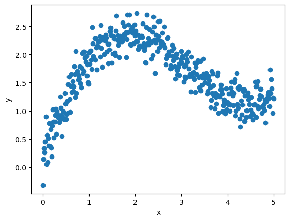
Now we generate some data to train the model.

x, y = generate_data()

Here’s a plot of the training data.

fig, ax = plt.subplots()
ax.scatter(x, y)
ax.set_xlabel('x')
ax.set_ylabel('y')
plt.show()

We’ll also use data from the same process for cross-validation.

x_validate, y_validate = generate_data()

22.2. Models

We supply functions to build two types of models.

22.3. Regression model

The first implements linear regression.

This is achieved by constructing a neural network with just one layer, that maps to a single dimension (since the prediction is real-valued).

The object model will be an instance of keras.Sequential, which is used to group a stack of layers into a single prediction model.

def build_regression_model():
    # Generate an instance of Sequential, to store layers and training attributes
    model = Sequential()
    # Add a single layer with scalar output
    model.add(Dense(units=1))  
    # Configure the model for training
    model.compile(optimizer=keras.optimizers.SGD(), 
                  loss='mean_squared_error')
    return model

In the function above you can see that

• we use stochastic gradient descent to train the model, and

• the loss is mean squared error (MSE).

The call model.add adds a single layer the activation function equal to the identity map.

MSE is the standard loss function for ordinary least squares regression.

22.3.1. Deep Network

The second function creates a dense (i.e., fully connected) neural network with 3 hidden layers, where each hidden layer maps to a k-dimensional output space.

def build_nn_model(output_dim=10, num_layers=3, activation_function='tanh'):
    # Create a Keras Model instance using Sequential()
    model = Sequential()
    # Add layers to the network sequentially, from inputs towards outputs
    for i in range(num_layers):
        model.add(Dense(units=output_dim, activation=activation_function))
    # Add a final layer that maps to a scalar value, for regression.
    model.add(Dense(units=1))
    # Embed training configurations
    model.compile(optimizer=keras.optimizers.SGD(), 
                  loss='mean_squared_error')
    return model

22.3.2. Tracking errors

The following function will be used to plot the MSE of the model during the training process.

Initially the MSE will be relatively high, but it should fall at each iteration, as the parameters are adjusted to better fit the data.

def plot_loss_history(training_history, ax):
    # Plot MSE of training data against epoch
    epochs = training_history.epoch
    ax.plot(epochs, 
            np.array(training_history.history['loss']), 
            label='training loss')
    # Plot MSE of validation data against epoch
    ax.plot(epochs, 
            np.array(training_history.history['val_loss']),
            label='validation loss')
    # Add labels
    ax.set_xlabel('Epoch')
    ax.set_ylabel('Loss (Mean squared error)')
    ax.legend()

22.4. Training

Now let’s go ahead and train our models.

22.4.1. Linear regression

We’ll start with linear regression.

regression_model = build_regression_model()

Now we train the model using the training data.

training_history = regression_model.fit(
    x, y, batch_size=x.shape[0], verbose=0,
    epochs=2000, validation_data=(x_validate, y_validate))

Let’s have a look at the evolution of MSE as the model is trained.

fig, ax = plt.subplots()
plot_loss_history(training_history, ax)
plt.show()

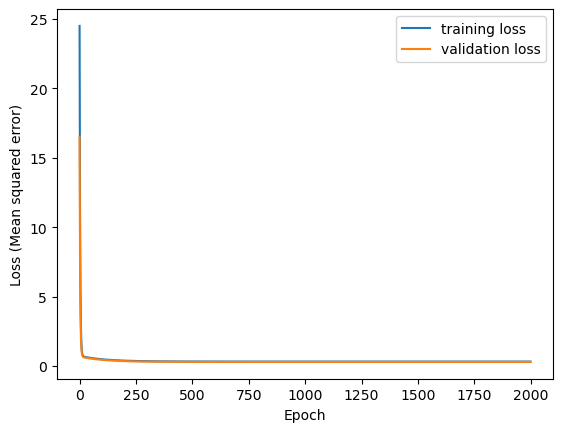
Let’s print the final MSE on the cross-validation data.

print("Testing loss on the validation set.")
regression_model.evaluate(x_validate, y_validate, verbose=2)

Testing loss on the validation set.
13/13 - 0s - 13ms/step - loss: 0.3016

0.3015977740287781

Here’s our output predictions on the cross-validation data.

y_predict = regression_model.predict(x_validate, verbose=2)

13/13 - 0s - 5ms/step

We use the following function to plot our predictions along with the data.

def plot_results(x, y, y_predict, ax):
    ax.scatter(x, y)
    ax.plot(x, y_predict, label="fitted model", color='black')
    ax.set_xlabel('x')
    ax.set_ylabel('y')

Let’s now call the function on the cross-validation data.

fig, ax = plt.subplots()
plot_results(x_validate, y_validate, y_predict, ax)
plt.show()

22.4.2. Deep learning

Now let’s switch to a neural network with multiple layers.

We implement the same steps as before.

nn_model = build_nn_model()

training_history = nn_model.fit(
    x, y, batch_size=x.shape[0], verbose=0,
    epochs=2000, validation_data=(x_validate, y_validate))

fig, ax = plt.subplots()
plot_loss_history(training_history, ax)
plt.show()

Here’s the final MSE for the deep learning model.

print("Testing loss on the validation set.")
nn_model.evaluate(x_validate, y_validate, verbose=2)

Testing loss on the validation set.

13/13 - 0s - 26ms/step - loss: 0.0432

0.04316260293126106

You will notice that this loss is much lower than the one we achieved with linear regression, suggesting a better fit.

To confirm this, let’s look at the fitted function.

y_predict = nn_model.predict(x_validate, verbose=2)

13/13 - 0s - 10ms/step

def plot_results(x, y, y_predict, ax):
    ax.scatter(x, y)
    ax.plot(x, y_predict, label="fitted model", color='black')
    ax.set_xlabel('x')
    ax.set_ylabel('y')

fig, ax = plt.subplots()
plot_results(x_validate, y_validate, y_predict, ax)
plt.show()

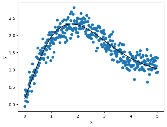
Not surprisingly, the multilayer neural network does a much better job of fitting the data.

In a a follow-up lecture, we will try to achieve the same fit using pure JAX, rather than relying on the Keras front-end.