21. Maximum Likelihood Estimation#
GPU
This lecture was built using a machine with access to a GPU — although it will also run without one.
Google Colab has a free tier with GPUs that you can access as follows:
Click on the “play” icon top right
Select Colab
Set the runtime environment to include a GPU
21.1. Overview#
This lecture is the extended JAX implementation of this section of this lecture.
Please refer that lecture for all background and notation.
Here we will exploit the automatic differentiation capabilities of JAX rather than calculating derivatives by hand.
We’ll require the following imports:
import matplotlib.pyplot as plt
from collections import namedtuple
import jax.numpy as jnp
import jax
from statsmodels.api import Poisson
Let’s check the GPU we are running
!nvidia-smi
Thu Jul  9 05:42:25 2026
+-----------------------------------------------------------------------------------------+
| NVIDIA-SMI 580.105.08             Driver Version: 580.105.08     CUDA Version: 13.0     |
+-----------------------------------------+------------------------+----------------------+
| GPU  Name                 Persistence-M | Bus-Id          Disp.A | Volatile Uncorr. ECC |
| Fan  Temp   Perf          Pwr:Usage/Cap |           Memory-Usage | GPU-Util  Compute M. |
|                                         |                        |               MIG M. |
|=========================================+========================+======================|
|   0  Tesla T4                       On  |   00000000:00:1E.0 Off |                    0 |
| N/A   37C    P0             26W /   70W |       0MiB /  15360MiB |      0%      Default |
|                                         |                        |                  N/A |
+-----------------------------------------+------------------------+----------------------+

+-----------------------------------------------------------------------------------------+
| Processes:                                                                              |
|  GPU   GI   CI              PID   Type   Process name                        GPU Memory |
|        ID   ID                                                               Usage      |
|=========================================================================================|
|  No running processes found                                                             |
+-----------------------------------------------------------------------------------------+
We will use 64 bit floats with JAX in order to increase the precision.
jax.config.update("jax_enable_x64", True)
21.2. MLE with numerical methods (JAX)#
Many distributions do not have nice, analytical solutions and therefore require numerical methods to solve for parameter estimates.
One such numerical method is the Newton-Raphson algorithm.
Let’s start with a simple example to illustrate the algorithm.
21.2.1. A toy model#
Our goal is to find the maximum likelihood estimate \(\hat{\boldsymbol{\beta}}\).
At \(\hat{\boldsymbol{\beta}}\), the first derivative of the log-likelihood function will be equal to 0.
Let’s illustrate this by supposing
Define the function logL.
@jax.jit
def logL(β):
    return -(β - 10) ** 2 - 10
To find the value of \(\frac{d \log \mathcal{L(\boldsymbol{\beta})}}{d \boldsymbol{\beta}}\), we can use jax.grad which auto-differentiates the given function.
We further use jax.vmap which vectorizes the given function i.e. the function acting upon scalar inputs can now be used with vector inputs.
dlogL = jax.vmap(jax.grad(logL))
β = jnp.linspace(1, 20)

fig, (ax1, ax2) = plt.subplots(2, sharex=True, figsize=(12, 8))

ax1.plot(β, logL(β), lw=2)
ax2.plot(β, dlogL(β), lw=2)

ax1.set_ylabel(r'$log \mathcal{L(\beta)}$',
               rotation=0,
               labelpad=35,
               fontsize=15)
ax2.set_ylabel(r'$\frac{dlog \mathcal{L(\beta)}}{d \beta}$ ',
               rotation=0,
               labelpad=35,
               fontsize=19)

ax2.set_xlabel(r'$\beta$', fontsize=15)
ax1.grid(), ax2.grid()
plt.axhline(c='black')
plt.show()
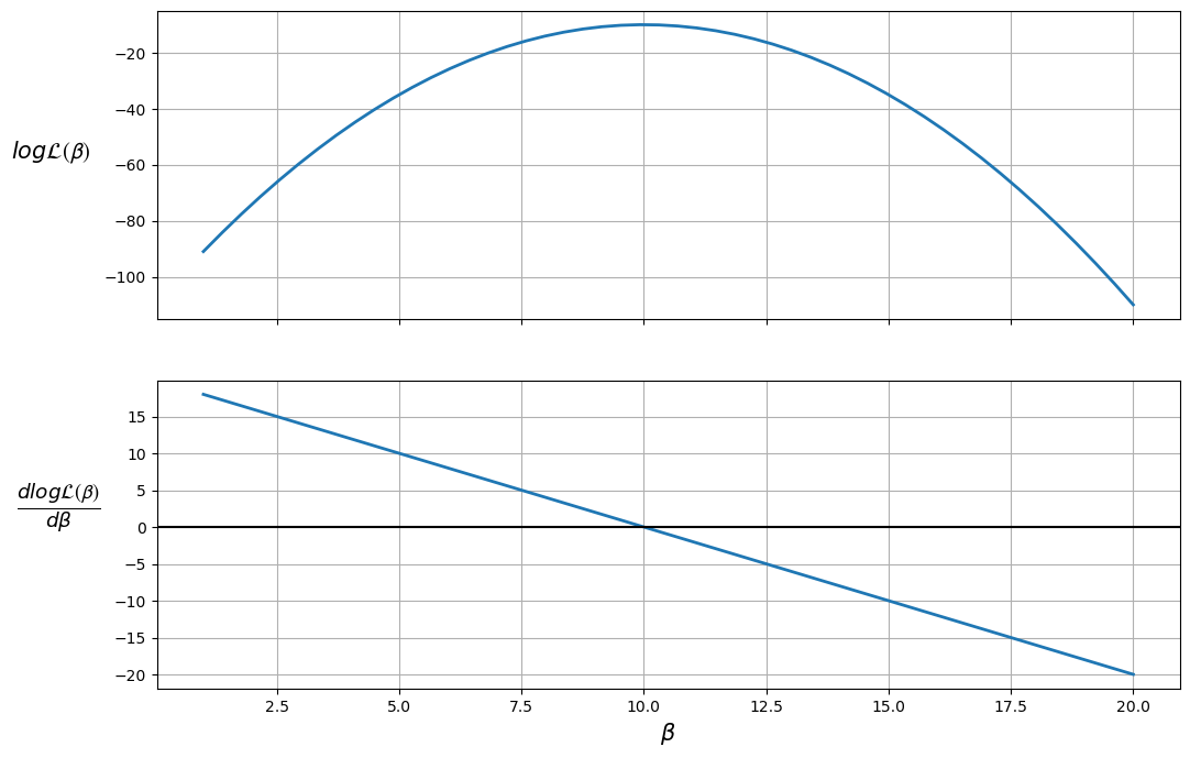
The plot shows that the maximum likelihood value (the top plot) occurs when \(\frac{d \log \mathcal{L(\boldsymbol{\beta})}}{d \boldsymbol{\beta}} = 0\) (the bottom plot).
Therefore, the likelihood is maximized when \(\beta = 10\).
We can also ensure that this value is a maximum (as opposed to a minimum) by checking that the second derivative (slope of the bottom plot) is negative.
The Newton-Raphson algorithm finds a point where the first derivative is 0.
To use the algorithm, we take an initial guess at the maximum value, \(\beta_0\) (the OLS parameter estimates might be a reasonable guess).
Then we use the updating rule involving gradient information to iterate the algorithm until the error is sufficiently small or the algorithm reaches the maximum number of iterations.
Please refer to this section for the detailed algorithm.
21.2.2. A Poisson model#
Let’s have a go at implementing the Newton-Raphson algorithm to calculate the maximum likelihood estimations of a Poisson regression.
The Poisson regression has a joint pmf:
We create a namedtuple to store the observed values
RegressionModel = namedtuple('RegressionModel', ['X', 'y'])

def create_regression_model(X, y):
    n, k = X.shape
    # Reshape y as a n_by_1 column vector
    y = y.reshape(n, 1)
    X, y = jax.device_put((X, y))
    return RegressionModel(X=X, y=y)
The log likelihood function of the Poisson regression is
The full derivation can be found here.
The log likelihood function involves factorial, but JAX doesn’t have a readily available implementation to compute factorial directly.
In order to compute the factorial efficiently such that we can JIT it, we use
since jax.lax.lgamma and jax.lax.exp are available.
The following function jax_factorial computes the factorial using this idea.
Let’s define this function in Python
@jax.jit
def _factorial(n):
    return jax.lax.exp(jax.lax.lgamma(n + 1.0)).astype(int)

jax_factorial = jax.vmap(_factorial)
Now we can define the log likelihood function in Python
@jax.jit
def poisson_logL(β, model):
    y = model.y
    μ = jnp.exp(model.X @ β)
    return jnp.sum(model.y * jnp.log(μ) - μ - jnp.log(jax_factorial(y)))
To find the gradient of the poisson_logL, we again use jax.grad.
According to the documentation,
jax.jacfwduses forward-mode automatic differentiation, which is more efficient for “tall” Jacobian matrices, whilejax.jacrevuses reverse-mode, which is more efficient for “wide” Jacobian matrices.
(The documentation also states that when matrices that are near-square, jax.jacfwd probably has an edge over jax.jacrev.)
Therefore, to find the Hessian, we can directly use jax.jacfwd.
G_poisson_logL = jax.grad(poisson_logL)
H_poisson_logL = jax.jacfwd(G_poisson_logL)
Our function newton_raphson will take a RegressionModel object
that has an initial guess of the parameter vector \(\boldsymbol{\beta}_0\).
The algorithm will update the parameter vector according to the updating rule, and recalculate the gradient and Hessian matrices at the new parameter estimates.
def newton_raphson(model, β, tol=1e-3, max_iter=100, display=True):

    i = 0
    error = 100  # Initial error value

    # Print header of output
    if display:
        header = f'{"Iteration_k":<13}{"Log-likelihood":<16}{"θ":<60}'
        print(header)
        print("-" * len(header))

    # While loop runs while any value in error is greater
    # than the tolerance until max iterations are reached
    while jnp.any(error > tol) and i < max_iter:
        H, G = jnp.squeeze(H_poisson_logL(β, model)), G_poisson_logL(β, model)
        β_new = β - (jnp.dot(jnp.linalg.inv(H), G))
        error = jnp.abs(β_new - β)
        β = β_new

        if display:
            β_list = [f'{t:.3}' for t in list(β.flatten())]
            update = f'{i:<13}{poisson_logL(β, model):<16.8}{β_list}'
            print(update)

        i += 1

    print(f'Number of iterations: {i}')
    print(f'β_hat = {β.flatten()}')

    return β
Let’s try out our algorithm with a small dataset of 5 observations and 3 variables in \(\mathbf{X}\).
X = jnp.array([[1, 2, 5],
               [1, 1, 3],
               [1, 4, 2],
               [1, 5, 2],
               [1, 3, 1]])

y = jnp.array([1, 0, 1, 1, 0])

# Take a guess at initial βs
init_β = jnp.array([0.1, 0.1, 0.1]).reshape(X.shape[1], 1)

# Create an object with Poisson model values
poi = create_regression_model(X, y)

# Use newton_raphson to find the MLE
β_hat = newton_raphson(poi, init_β, display=True)
Iteration_k  Log-likelihood  θ
-----------------------------------------------------------------------------------------
0            -4.3447622      ['-1.49', '0.265', '0.244']
1            -3.5742413      ['-3.38', '0.528', '0.474']
2            -3.3999526      ['-5.06', '0.782', '0.702']
3            -3.3788646      ['-5.92', '0.909', '0.82']
4            -3.3783559      ['-6.07', '0.933', '0.843']
5            -3.3783555      ['-6.08', '0.933', '0.843']
6            -3.3783555      ['-6.08', '0.933', '0.843']
Number of iterations: 7
β_hat = [-6.07848573  0.9334028   0.84329677]
As this was a simple model with few observations, the algorithm achieved convergence in only 7 iterations.
The gradient vector should be close to 0 at \(\hat{\boldsymbol{\beta}}\)
G_poisson_logL(β_hat, poi)
Array([[-2.53297383e-13],
       [-6.40432152e-13],
       [-4.93882713e-13]], dtype=float64)
21.3. MLE with statsmodels#
We’ll use the Poisson regression model in statsmodels to verify the results
obtained using JAX.
statsmodels uses the same algorithm as above to find the maximum
likelihood estimates.
Now, as statsmodels accepts only NumPy arrays, we can use the __array__ method
of JAX arrays to convert it to NumPy arrays.
X_numpy = X.__array__()
y_numpy = y.__array__()
stats_poisson = Poisson(y_numpy, X_numpy).fit()
print(stats_poisson.summary())
Optimization terminated successfully.
         Current function value: 0.675671
         Iterations 7
                          Poisson Regression Results
==============================================================================
Dep. Variable:                      y   No. Observations:                    5
Model:                        Poisson   Df Residuals:                        2
Method:                           MLE   Df Model:                            2
Date:                Thu, 09 Jul 2026   Pseudo R-squ.:                  0.2546
Time:                        05:42:28   Log-Likelihood:                -3.3784
converged:                       True   LL-Null:                       -4.5325
Covariance Type:            nonrobust   LLR p-value:                    0.3153
==============================================================================
                 coef    std err          z      P>|z|      [0.025      0.975]
------------------------------------------------------------------------------
const         -6.0785      5.279     -1.151      0.250     -16.425       4.268
x1             0.9334      0.829      1.126      0.260      -0.691       2.558
x2             0.8433      0.798      1.057      0.291      -0.720       2.407
==============================================================================
The benefit of writing our own procedure, relative to statsmodels is that
we can exploit the power of the GPU and
we learn the underlying methodology, which can be extended to complex situations where no existing routines are available.
Exercise 21.1
We define a quadratic model for a single explanatory variable by
We calculate the mean on the original scale instead of the log scale by exponentiating both sides of the above equation, which gives
Simulate the values of \(x_t\) by sampling from a normal distribution and \(\lambda_t\) by using (21.1) and the following constants:
Try to obtain the approximate values of \(\beta_0,\beta_1,\beta_2\), by simulating a Poisson Regression Model such that
Using our newton_raphson function on the data set \(X = [1, x_t, x_t^{2}]\) and
\(y\), obtain the maximum likelihood estimates of \(\beta_0,\beta_1,\beta_2\).
With a sufficient large sample size, you should approximately recover the true values of of these parameters.
Solution
Let’s start by defining “true” parameter values.
β_0 = -2.5
β_1 = 0.25
β_2 = 0.5
To simulate the model, we sample 500,000 values of \(x_t\) from the standard normal distribution.
seed = 32
shape = (500_000, 1)
key = jax.random.key(seed)
x = jax.random.normal(key, shape)
We compute \(\lambda\) using (21.1)
λ = jnp.exp(β_0 + β_1 * x + β_2 * x**2)
Let’s define \(y_t\) by sampling from a Poisson distribution with mean as \(\lambda_t\).
y = jax.random.poisson(key, λ, shape)
Now let’s try to recover the true parameter values using the Newton-Raphson method described above.
X = jnp.hstack((jnp.ones(shape), x, x**2))

# Take a guess at initial βs
init_β = jnp.array([0.1, 0.1, 0.1]).reshape(X.shape[1], 1)

# Create an object with Poisson model values
poi = create_regression_model(X, y)

# Use newton_raphson to find the MLE
β_hat = newton_raphson(poi, init_β, tol=1e-5, display=True)
Iteration_k  Log-likelihood  θ
-----------------------------------------------------------------------------------------
0            -2.2775261e+08  ['-1.58', '0.338', '0.87']
1            -8.3204829e+07  ['-2.55', '0.338', '0.869']
2            -3.0152953e+07  ['-3.48', '0.338', '0.866']
3            -1.075084e+07   ['-4.29', '0.336', '0.856']
4            -3704112.6      ['-4.81', '0.333', '0.832']
5            -1155469.9      ['-4.71', '0.324', '0.778']
6            -213241.4       ['-3.81', '0.307', '0.684']
7            124155.52       ['-2.99', '0.284', '0.596']
8            220518.05       ['-2.67', '0.266', '0.54']
9            236821.42       ['-2.54', '0.255', '0.509']
10           237651.75       ['-2.51', '0.252', '0.5']
11           237654.97       ['-2.5', '0.252', '0.5']
12           237654.97       ['-2.5', '0.252', '0.5']
Number of iterations: 13
β_hat = [-2.50352915  0.25171711  0.49977956]
The maximum likelihood estimates are similar to the true parameter values.