14. Optimal Investment#

GPU

This lecture was built using a machine with JAX installed and access to a GPU.

To run this lecture on Google Colab, click on the “play” icon top right, select Colab, and set the runtime environment to include a GPU.

To run this lecture on your own machine, you need to install Google JAX.

In addition to JAX and Anaconda, this lecture will need the following libraries:

!pip install --upgrade quantecon

Show code cell output Hide code cell output

Requirement already satisfied: quantecon in /opt/conda/envs/quantecon/lib/python3.12/site-packages (0.7.2)

Requirement already satisfied: numba>=0.49.0 in /opt/conda/envs/quantecon/lib/python3.12/site-packages (from quantecon) (0.60.0)
Requirement already satisfied: numpy>=1.17.0 in /opt/conda/envs/quantecon/lib/python3.12/site-packages (from quantecon) (1.26.4)
Requirement already satisfied: requests in /opt/conda/envs/quantecon/lib/python3.12/site-packages (from quantecon) (2.32.3)
Requirement already satisfied: scipy>=1.5.0 in /opt/conda/envs/quantecon/lib/python3.12/site-packages (from quantecon) (1.13.1)
Requirement already satisfied: sympy in /opt/conda/envs/quantecon/lib/python3.12/site-packages (from quantecon) (1.13.2)
Requirement already satisfied: llvmlite<0.44,>=0.43.0dev0 in /opt/conda/envs/quantecon/lib/python3.12/site-packages (from numba>=0.49.0->quantecon) (0.43.0)
Requirement already satisfied: charset-normalizer<4,>=2 in /opt/conda/envs/quantecon/lib/python3.12/site-packages (from requests->quantecon) (3.3.2)
Requirement already satisfied: idna<4,>=2.5 in /opt/conda/envs/quantecon/lib/python3.12/site-packages (from requests->quantecon) (3.7)
Requirement already satisfied: urllib3<3,>=1.21.1 in /opt/conda/envs/quantecon/lib/python3.12/site-packages (from requests->quantecon) (2.2.3)
Requirement already satisfied: certifi>=2017.4.17 in /opt/conda/envs/quantecon/lib/python3.12/site-packages (from requests->quantecon) (2024.8.30)
Requirement already satisfied: mpmath<1.4,>=1.1.0 in /opt/conda/envs/quantecon/lib/python3.12/site-packages (from sympy->quantecon) (1.3.0)

WARNING: Running pip as the 'root' user can result in broken permissions and conflicting behaviour with the system package manager, possibly rendering your system unusable.It is recommended to use a virtual environment instead: https://pip.pypa.io/warnings/venv. Use the --root-user-action option if you know what you are doing and want to suppress this warning.

We study a monopolist who faces inverse demand curve

\[ P_t = a_0 - a_1 Y_t + Z_t, \]

where

\(P_t\) is price,
\(Y_t\) is output and
\(Z_t\) is a demand shock.

We assume that \(Z_t\) is a discretized AR(1) process, specified below.

Current profits are

\[ P_t Y_t - c Y_t - \gamma (Y_{t+1} - Y_t)^2 \]

Combining with the demand curve and writing \(y, y'\) for \(Y_t, Y_{t+1}\), this becomes

\[ r(y, z, y') := (a_0 - a_1 y + z - c) y - γ (y' - y)^2 \]

The firm maximizes present value of expected discounted profits. The Bellman equation is

\[ v(y, z) = \max_{y'} \left\{ r(y, z, y') + β \sum_{z'} v(y', z') Q(z, z') \right\}. \]

We discretize \(y\) to a finite grid y_grid.

In essence, the firm tries to choose output close to the monopolist profit maximizer, given \(Z_t\), but is constrained by adjustment costs.

Let’s begin with the following imports

import quantecon as qe
import jax
import jax.numpy as jnp
import matplotlib.pyplot as plt
from time import time

Let’s check the GPU we are running

!nvidia-smi

Mon Feb 10 03:52:42 2025       
+-----------------------------------------------------------------------------------------+
| NVIDIA-SMI 550.127.05             Driver Version: 550.127.05     CUDA Version: 12.4     |
|-----------------------------------------+------------------------+----------------------+
| GPU  Name                 Persistence-M | Bus-Id          Disp.A | Volatile Uncorr. ECC |
| Fan  Temp   Perf          Pwr:Usage/Cap |           Memory-Usage | GPU-Util  Compute M. |
|                                         |                        |               MIG M. |
|=========================================+========================+======================|
|   0  Tesla T4                       On  |   00000001:00:00.0 Off |                  Off |
| N/A   38C    P8              9W /   70W |       1MiB /  16384MiB |      0%      Default |
|                                         |                        |                  N/A |
+-----------------------------------------+------------------------+----------------------+
                                                                                         
+-----------------------------------------------------------------------------------------+
| Processes:                                                                              |
|  GPU   GI   CI        PID   Type   Process name                              GPU Memory |
|        ID   ID                                                               Usage      |
|=========================================================================================|
|  No running processes found                                                             |
+-----------------------------------------------------------------------------------------+

We will use 64 bit floats with JAX in order to increase the precision.

jax.config.update("jax_enable_x64", True)

Let’s define a function to create an investment model using the given parameters.

def create_investment_model(
        r=0.01,                              # Interest rate
        a_0=10.0, a_1=1.0,                   # Demand parameters
        γ=25.0, c=1.0,                       # Adjustment and unit cost
        y_min=0.0, y_max=20.0, y_size=100,   # Grid for output
        ρ=0.9, ν=1.0,                        # AR(1) parameters
        z_size=150):                         # Grid size for shock
    """
    A function that takes in parameters and returns an instance of Model that
    contains data for the investment problem.
    """
    β = 1 / (1 + r)
    y_grid = jnp.linspace(y_min, y_max, y_size)
    mc = qe.tauchen(z_size, ρ, ν)
    z_grid, Q = mc.state_values, mc.P

    # Break up parameters into static and nonstatic components
    constants = β, a_0, a_1, γ, c
    sizes = y_size, z_size
    arrays = y_grid, z_grid, Q

    # Shift arrays to the device (e.g., GPU)
    arrays = tuple(map(jax.device_put, arrays))
    return constants, sizes, arrays

Let’s re-write the vectorized version of the right-hand side of the Bellman equation (before maximization), which is a 3D array representing

\[ B(y, z, y') = r(y, z, y') + \beta \sum_{z'} v(y', z') Q(z, z') \]

for all \((y, z, y')\).

def B(v, constants, sizes, arrays):
    """
    A vectorized version of the right-hand side of the Bellman equation
    (before maximization)
    """

    # Unpack
    β, a_0, a_1, γ, c = constants
    y_size, z_size = sizes
    y_grid, z_grid, Q = arrays

    # Compute current rewards r(y, z, yp) as array r[i, j, ip]
    y  = jnp.reshape(y_grid, (y_size, 1, 1))    # y[i]   ->  y[i, j, ip]
    z  = jnp.reshape(z_grid, (1, z_size, 1))    # z[j]   ->  z[i, j, ip]
    yp = jnp.reshape(y_grid, (1, 1, y_size))    # yp[ip] -> yp[i, j, ip]
    r = (a_0 - a_1 * y + z - c) * y - γ * (yp - y)**2

    # Calculate continuation rewards at all combinations of (y, z, yp)
    v = jnp.reshape(v, (1, 1, y_size, z_size))  # v[ip, jp] -> v[i, j, ip, jp]
    Q = jnp.reshape(Q, (1, z_size, 1, z_size))  # Q[j, jp]  -> Q[i, j, ip, jp]
    EV = jnp.sum(v * Q, axis=3)                 # sum over last index jp

    # Compute the right-hand side of the Bellman equation
    return r + β * EV

# Create a jitted function
B = jax.jit(B, static_argnums=(2,))

We define a function to compute the current rewards \(r_\sigma\) given policy \(\sigma\), which is defined as the vector

\[ r_\sigma(y, z) := r(y, z, \sigma(y, z)) \]

def compute_r_σ(σ, constants, sizes, arrays):
    """
    Compute the array r_σ[i, j] = r[i, j, σ[i, j]], which gives current
    rewards given policy σ.
    """

    # Unpack model
    β, a_0, a_1, γ, c = constants
    y_size, z_size = sizes
    y_grid, z_grid, Q = arrays

    # Compute r_σ[i, j]
    y = jnp.reshape(y_grid, (y_size, 1))
    z = jnp.reshape(z_grid, (1, z_size))
    yp = y_grid[σ]
    r_σ = (a_0 - a_1 * y + z - c) * y - γ * (yp - y)**2

    return r_σ


# Create the jitted function
compute_r_σ = jax.jit(compute_r_σ, static_argnums=(2,))

Define the Bellman operator.

def T(v, constants, sizes, arrays):
    """The Bellman operator."""
    return jnp.max(B(v, constants, sizes, arrays), axis=2)

T = jax.jit(T, static_argnums=(2,))

The following function computes a v-greedy policy.

def get_greedy(v, constants, sizes, arrays):
    "Computes a v-greedy policy, returned as a set of indices."
    return jnp.argmax(B(v, constants, sizes, arrays), axis=2)

get_greedy = jax.jit(get_greedy, static_argnums=(2,))

Define the \(\sigma\)-policy operator.

def T_σ(v, σ, constants, sizes, arrays):
    """The σ-policy operator."""

    # Unpack model
    β, a_0, a_1, γ, c = constants
    y_size, z_size = sizes
    y_grid, z_grid, Q = arrays

    r_σ = compute_r_σ(σ, constants, sizes, arrays)

    # Compute the array v[σ[i, j], jp]
    zp_idx = jnp.arange(z_size)
    zp_idx = jnp.reshape(zp_idx, (1, 1, z_size))
    σ = jnp.reshape(σ, (y_size, z_size, 1))
    V = v[σ, zp_idx]

    # Convert Q[j, jp] to Q[i, j, jp]
    Q = jnp.reshape(Q, (1, z_size, z_size))

    # Calculate the expected sum Σ_jp v[σ[i, j], jp] * Q[i, j, jp]
    Ev = jnp.sum(V * Q, axis=2)

    return r_σ + β * Ev

T_σ = jax.jit(T_σ, static_argnums=(3,))

Next, we want to computes the lifetime value of following policy \(\sigma\).

This lifetime value is a function \(v_\sigma\) that satisfies

\[ v_\sigma(y, z) = r_\sigma(y, z) + \beta \sum_{z'} v_\sigma(\sigma(y, z), z') Q(z, z') \]

We wish to solve this equation for \(v_\sigma\).

Suppose we define the linear operator \(L_\sigma\) by

\[ (L_\sigma v)(y, z) = v(y, z) - \beta \sum_{z'} v(\sigma(y, z), z') Q(z, z') \]

With this notation, the problem is to solve for \(v\) via

\[ (L_{\sigma} v)(y, z) = r_\sigma(y, z) \]

In vector for this is \(L_\sigma v = r_\sigma\), which tells us that the function we seek is

\[ v_\sigma = L_\sigma^{-1} r_\sigma \]

JAX allows us to solve linear systems defined in terms of operators; the first step is to define the function \(L_{\sigma}\).

def L_σ(v, σ, constants, sizes, arrays):

    β, a_0, a_1, γ, c = constants
    y_size, z_size = sizes
    y_grid, z_grid, Q = arrays

    # Set up the array v[σ[i, j], jp]
    zp_idx = jnp.arange(z_size)
    zp_idx = jnp.reshape(zp_idx, (1, 1, z_size))
    σ = jnp.reshape(σ, (y_size, z_size, 1))
    V = v[σ, zp_idx]

    # Expand Q[j, jp] to Q[i, j, jp]
    Q = jnp.reshape(Q, (1, z_size, z_size))

    # Compute and return v[i, j] - β Σ_jp v[σ[i, j], jp] * Q[j, jp]
    return v - β * jnp.sum(V * Q, axis=2)

L_σ = jax.jit(L_σ, static_argnums=(3,))

Now we can define a function to compute \(v_{\sigma}\)

def get_value(σ, constants, sizes, arrays):

    # Unpack
    β, a_0, a_1, γ, c = constants
    y_size, z_size = sizes
    y_grid, z_grid, Q = arrays

    r_σ = compute_r_σ(σ, constants, sizes, arrays)

    # Reduce L_σ to a function in v
    partial_L_σ = lambda v: L_σ(v, σ, constants, sizes, arrays)

    return jax.scipy.sparse.linalg.bicgstab(partial_L_σ, r_σ)[0]

get_value = jax.jit(get_value, static_argnums=(2,))

We use successive approximation for VFI.

def successive_approx_jax(T,                     # Operator (callable)
                          x_0,                   # Initial condition                
                          tol=1e-6,              # Error tolerance
                          max_iter=10_000):      # Max iteration bound
    def body_fun(k_x_err):
        k, x, error = k_x_err
        x_new = T(x)
        error = jnp.max(jnp.abs(x_new - x))
        return k + 1, x_new, error

    def cond_fun(k_x_err):
        k, x, error = k_x_err
        return jnp.logical_and(error > tol, k < max_iter)

    k, x, error = jax.lax.while_loop(cond_fun, body_fun, (1, x_0, tol + 1))
    return x

successive_approx_jax = jax.jit(successive_approx_jax, static_argnums=(0,))

For OPI we’ll add a compiled routine that computes \(T_σ^m v\).

def iterate_policy_operator(σ, v, m, params, sizes, arrays):

    def update(i, v):
        v = T_σ(v, σ, params, sizes, arrays)
        return v
    
    v = jax.lax.fori_loop(0, m, update, v)
    return v

iterate_policy_operator = jax.jit(iterate_policy_operator,
                                  static_argnums=(4,))

Finally, we introduce the solvers that implement VFI, HPI and OPI.

def value_function_iteration(model, tol=1e-5):
    """
    Implements value function iteration.
    """
    params, sizes, arrays = model
    vz = jnp.zeros(sizes)
    _T = lambda v: T(v, params, sizes, arrays)
    v_star = successive_approx_jax(_T, vz, tol=tol)
    return get_greedy(v_star, params, sizes, arrays)

For OPI we will use a compiled JAX lax.while_loop operation to speed execution.

def opi_loop(params, sizes, arrays, m, tol, max_iter):
    """
    Implements optimistic policy iteration (see dp.quantecon.org) with 
    step size m.

    """
    v_init = jnp.zeros(sizes)

    def condition_function(inputs):
        i, v, error = inputs
        return jnp.logical_and(error > tol, i < max_iter)

    def update(inputs):
        i, v, error = inputs
        last_v = v
        σ = get_greedy(v, params, sizes, arrays)
        v = iterate_policy_operator(σ, v, m, params, sizes, arrays)
        error = jnp.max(jnp.abs(v - last_v))
        i += 1
        return i, v, error

    num_iter, v, error = jax.lax.while_loop(condition_function,
                                            update,
                                            (0, v_init, tol + 1))

    return get_greedy(v, params, sizes, arrays)

opi_loop = jax.jit(opi_loop, static_argnums=(1,))

Here’s a friendly interface to OPI

def optimistic_policy_iteration(model, m=10, tol=1e-5, max_iter=10_000):
    params, sizes, arrays = model
    σ_star = opi_loop(params, sizes, arrays, m, tol, max_iter)
    return σ_star

Here’s HPI

def howard_policy_iteration(model, maxiter=250):
    """
    Implements Howard policy iteration (see dp.quantecon.org)
    """
    params, sizes, arrays = model
    σ = jnp.zeros(sizes, dtype=int)
    i, error = 0, 1.0
    while error > 0 and i < maxiter:
        v_σ = get_value(σ, params, sizes, arrays)
        σ_new = get_greedy(v_σ, params, sizes, arrays)
        error = jnp.max(jnp.abs(σ_new - σ))
        σ = σ_new
        i = i + 1
        print(f"Concluded loop {i} with error {error}.")
    return σ

model = create_investment_model()
constants, sizes, arrays = model
β, a_0, a_1, γ, c = constants
y_size, z_size = sizes
y_grid, z_grid, Q = arrays

print("Starting HPI.")
%time σ_star_hpi = howard_policy_iteration(model).block_until_ready()

# Now time it without compile time
start = time()
σ_star_hpi = howard_policy_iteration(model).block_until_ready()
hpi_without_compile = time() - start
print(σ_star_hpi)
print(f"HPI completed in {hpi_without_compile} seconds.")

Concluded loop 1 with error 50.
Concluded loop 2 with error 26.
Concluded loop 3 with error 17.
Concluded loop 4 with error 10.
Concluded loop 5 with error 7.

Concluded loop 6 with error 4.
Concluded loop 7 with error 3.
Concluded loop 8 with error 1.
Concluded loop 9 with error 1.
Concluded loop 10 with error 1.
Concluded loop 11 with error 1.
Concluded loop 12 with error 0.
[[ 2  2  2 ...  6  6  6]
 [ 3  3  3 ...  7  7  7]
 [ 4  4  4 ...  7  7  7]
 ...
 [82 82 82 ... 86 86 86]
 [83 83 83 ... 86 86 86]
 [84 84 84 ... 87 87 87]]
HPI completed in 0.11818718910217285 seconds.

Here’s the plot of the Howard policy, as a function of \(y\) at the highest and lowest values of \(z\).

fig, ax = plt.subplots(figsize=(9, 5))
ax.plot(y_grid, y_grid, "k--", label="45")
ax.plot(y_grid, y_grid[σ_star_hpi[:, 1]], label="$\\sigma^{*}_{HPI}(\cdot, z_1)$")
ax.plot(y_grid, y_grid[σ_star_hpi[:, -1]], label="$\\sigma^{*}_{HPI}(\cdot, z_N)$")
ax.legend(fontsize=12)
plt.show()

<>:3: SyntaxWarning: invalid escape sequence '\c'
<>:4: SyntaxWarning: invalid escape sequence '\c'
<>:3: SyntaxWarning: invalid escape sequence '\c'
<>:4: SyntaxWarning: invalid escape sequence '\c'
/tmp/ipykernel_2263/2467401157.py:3: SyntaxWarning: invalid escape sequence '\c'
  ax.plot(y_grid, y_grid[σ_star_hpi[:, 1]], label="$\\sigma^{*}_{HPI}(\cdot, z_1)$")
/tmp/ipykernel_2263/2467401157.py:4: SyntaxWarning: invalid escape sequence '\c'
  ax.plot(y_grid, y_grid[σ_star_hpi[:, -1]], label="$\\sigma^{*}_{HPI}(\cdot, z_N)$")

_images/6848b2edbadd317c88e9cbcb9258d3c0d5df6c9d2e54ab5fac6d6029f88e6013.png

print("Starting VFI.")
%time σ_star_vfi = value_function_iteration(model).block_until_ready()

# Now time it without compile time
start = time()
σ_star_vfi = value_function_iteration(model).block_until_ready()
vfi_without_compile = time() - start
print(σ_star_vfi)
print(f"VFI completed in {vfi_without_compile} seconds.")

[[ 2  2  2 ...  6  6  6]
 [ 3  3  3 ...  7  7  7]
 [ 4  4  4 ...  7  7  7]
 ...
 [82 82 82 ... 86 86 86]
 [83 83 83 ... 86 86 86]
 [84 84 84 ... 87 87 87]]
VFI completed in 0.49846553802490234 seconds.

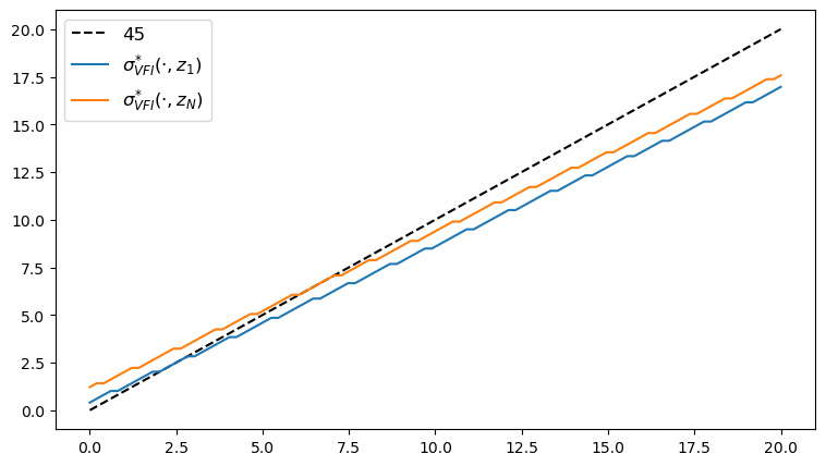
Here’s the plot of the VFI, as a function of \(y\) at the highest and lowest values of \(z\).

fig, ax = plt.subplots(figsize=(9, 5))
ax.plot(y_grid, y_grid, "k--", label="45")
ax.plot(y_grid, y_grid[σ_star_vfi[:, 1]], label="$\\sigma^{*}_{VFI}(\cdot, z_1)$")
ax.plot(y_grid, y_grid[σ_star_vfi[:, -1]], label="$\\sigma^{*}_{VFI}(\cdot, z_N)$")
ax.legend(fontsize=12)
plt.show()

<>:3: SyntaxWarning: invalid escape sequence '\c'
<>:4: SyntaxWarning: invalid escape sequence '\c'
<>:3: SyntaxWarning: invalid escape sequence '\c'
<>:4: SyntaxWarning: invalid escape sequence '\c'
/tmp/ipykernel_2263/2642608191.py:3: SyntaxWarning: invalid escape sequence '\c'
  ax.plot(y_grid, y_grid[σ_star_vfi[:, 1]], label="$\\sigma^{*}_{VFI}(\cdot, z_1)$")
/tmp/ipykernel_2263/2642608191.py:4: SyntaxWarning: invalid escape sequence '\c'
  ax.plot(y_grid, y_grid[σ_star_vfi[:, -1]], label="$\\sigma^{*}_{VFI}(\cdot, z_N)$")

_images/4050a83e012f3ebb79b933310e4e28976575e79714e11f9ac1def7dd8115906f.png

print("Starting OPI.")
%time σ_star_opi = optimistic_policy_iteration(model, m=100).block_until_ready()

# Now time it without compile time
start = time()
σ_star_opi = optimistic_policy_iteration(model, m=100).block_until_ready()
opi_without_compile = time() - start
print(σ_star_opi)
print(f"OPI completed in {opi_without_compile} seconds.")

[[ 2  2  2 ...  6  6  6]
 [ 3  3  3 ...  7  7  7]
 [ 4  4  4 ...  7  7  7]
 ...
 [82 82 82 ... 86 86 86]
 [83 83 83 ... 86 86 86]
 [84 84 84 ... 87 87 87]]
OPI completed in 0.2251429557800293 seconds.

Here’s the plot of the optimal policy, as a function of \(y\) at the highest and lowest values of \(z\).

fig, ax = plt.subplots(figsize=(9, 5))
ax.plot(y_grid, y_grid, "k--", label="45")
ax.plot(y_grid, y_grid[σ_star_opi[:, 1]], label="$\\sigma^{*}_{OPI}(\cdot, z_1)$")
ax.plot(y_grid, y_grid[σ_star_opi[:, -1]], label="$\\sigma^{*}_{OPI}(\cdot, z_N)$")
ax.legend(fontsize=12)
plt.show()

<>:3: SyntaxWarning: invalid escape sequence '\c'
<>:4: SyntaxWarning: invalid escape sequence '\c'
<>:3: SyntaxWarning: invalid escape sequence '\c'
<>:4: SyntaxWarning: invalid escape sequence '\c'
/tmp/ipykernel_2263/3367176246.py:3: SyntaxWarning: invalid escape sequence '\c'
  ax.plot(y_grid, y_grid[σ_star_opi[:, 1]], label="$\\sigma^{*}_{OPI}(\cdot, z_1)$")
/tmp/ipykernel_2263/3367176246.py:4: SyntaxWarning: invalid escape sequence '\c'
  ax.plot(y_grid, y_grid[σ_star_opi[:, -1]], label="$\\sigma^{*}_{OPI}(\cdot, z_N)$")

_images/30d79d533cdfd0fcd9e61a09ac98e40303c33d2d41670171fc386bc91f6faa17.png

We observe that all the solvers produce the same output from the above three plots.

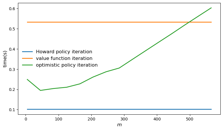
Let’s plot the time taken by each of the solvers and compare them.

m_vals = range(5, 600, 40)

print("Running Howard policy iteration.")
%time σ_hpi = howard_policy_iteration(model).block_until_ready()

Running Howard policy iteration.
Concluded loop 1 with error 50.
Concluded loop 2 with error 26.
Concluded loop 3 with error 17.
Concluded loop 4 with error 10.
Concluded loop 5 with error 7.
Concluded loop 6 with error 4.
Concluded loop 7 with error 3.
Concluded loop 8 with error 1.

Concluded loop 9 with error 1.
Concluded loop 10 with error 1.
Concluded loop 11 with error 1.
Concluded loop 12 with error 0.
CPU times: user 101 ms, sys: 9.69 ms, total: 111 ms
Wall time: 95.7 ms

# Now time it without compile time
start = time()
σ_hpi = howard_policy_iteration(model).block_until_ready()
hpi_without_compile = time() - start
print(f"HPI completed in {hpi_without_compile} seconds.")

Concluded loop 1 with error 50.
Concluded loop 2 with error 26.
Concluded loop 3 with error 17.
Concluded loop 4 with error 10.
Concluded loop 5 with error 7.
Concluded loop 6 with error 4.
Concluded loop 7 with error 3.
Concluded loop 8 with error 1.
Concluded loop 9 with error 1.
Concluded loop 10 with error 1.
Concluded loop 11 with error 1.
Concluded loop 12 with error 0.
HPI completed in 0.09476304054260254 seconds.

print("Running value function iteration.")
%time σ_vfi = value_function_iteration(model, tol=1e-5).block_until_ready()

Running value function iteration.

CPU times: user 498 ms, sys: 8.91 ms, total: 507 ms
Wall time: 501 ms

# Now time it without compile time
start = time()
σ_vfi = value_function_iteration(model, tol=1e-5).block_until_ready()
vfi_without_compile = time() - start
print(f"VFI completed in {vfi_without_compile} seconds.")

VFI completed in 0.4979712963104248 seconds.

opi_times = []
for m in m_vals:
    print(f"Running optimistic policy iteration with m={m}.")
    σ_opi = optimistic_policy_iteration(model, m=m, tol=1e-5).block_until_ready()

    # Now time it without compile time
    start = time()
    σ_opi = optimistic_policy_iteration(model, m=m, tol=1e-5).block_until_ready()
    opi_without_compile = time() - start
    print(f"OPI with m={m} completed in {opi_without_compile} seconds.")
    opi_times.append(opi_without_compile)

fig, ax = plt.subplots(figsize=(9, 5))
ax.plot(m_vals, jnp.full(len(m_vals), hpi_without_compile),
        lw=2, label="Howard policy iteration")
ax.plot(m_vals, jnp.full(len(m_vals), vfi_without_compile),
        lw=2, label="value function iteration")
ax.plot(m_vals, opi_times, lw=2, label="optimistic policy iteration")
ax.legend(fontsize=12, frameon=False)
ax.set_xlabel("$m$", fontsize=12)
ax.set_ylabel("time(s)", fontsize=12)
plt.show()

_images/59b2e6c453a22a23998029ca1a5a5dcf945ce9f2839fe5a0c70835bf06a0ddd5.png