24. Policy Gradient-Based Optimal Savings#
GPU
This lecture was built using a machine with access to a GPU — although it will also run without one.
Google Colab has a free tier with GPUs that you can access as follows:
Click on the “play” icon top right
Select Colab
Set the runtime environment to include a GPU
24.1. Introduction#
In this notebook we solve infinite horizon optimal savings problems using deep learning and policy gradient ascent with JAX.
Each policy is represented as a fully connected feed forward neural network.
We begin with a cake eating problem with a known analytical solution.
Then we shift to an income fluctuation problem where we can compute an optimal policy easily with the endogenous grid method (EGM).
We do this first and then try to learn the same policy with deep learning.
The technique we will use is called policy gradient ascent.
This method is popular in the machine learning community for solving high-dimensional dynamic programming problems.
Since the income fluctuation problem is low-dimensional, the policy gradient method will not be superior to EGM.
However, by working through this lecture, we can learn the basic principles of policy gradient methods and see them work in practice.
We’ll use the following libraries
!pip install optax
We’ll use the following imports
import jax
import jax.numpy as jnp
from jax import grad, jit, random
import optax
import matplotlib.pyplot as plt
from functools import partial
from typing import NamedTuple
24.2. Theory#
Let’s describe the income fluctuation problem and the ideas behind policy gradient ascent.
24.2.1. Household problem#
A household chooses a consumption plan \(\{c_t\}_{t \geq 0}\) to maximize
subject to
Here \(Y_t\) is labor income, which is IID and normally distributed:
We assume:
\(\beta R < 1\)
\(u\) is CRRA with parameter \(\gamma\)
We will be interested in the value of alternative policy functions for this household.
Since the shocks are IID, and hence offer no predictive content for future shocks, optimal policies will depend only on current assets.
The next section discusses policies and their values in more detail.
24.2.2. Lifetime Value and Optimization#
A policy is a function \(\sigma\) from \(\mathbb{R}_+\) to itself, where \(\sigma(a)\) is understood as the amount consumed under policy \(\sigma\) given current state \(a\).
A feasible policy is a (measurable) policy satisfying \(0 \leq \sigma(a) \leq a\) for all \(a\) (no borrowing).
We let \(\Sigma\) denote the set of all feasible policies.
We let \(v_\sigma(a)\) be the lifetime value of following policy \(\sigma\), given initial assets \(a\).
That is,
where
\(c_t = \sigma(a_t)\)
\(a_0 = a\)
\(a_{t+1} = R (a_t - \sigma(a_t)) + Y_{t+1}\) for \(t = 0, 1,\ldots\)
A policy \(\sigma\) is called optimal if \(v_s(a) \leq v_\sigma(a)\) for all asset levels \(a\) and all alternative policies \(s \in \Sigma\).
The function \(v^*\) defined by \(v^*(a) := \sup_{\sigma \in \Sigma} v_\sigma(a)\) is called the value function.
Using this definition, we can alternatively say that a policy \(\sigma\) is optimal if and only if \(v_\sigma = v^*\).
We know that we can find an optimal policy using dynamic programming and, in particular, the endogenous grid method (EGM).
Now let’s look at another method.
24.2.3. The policy gradient approach#
The policy gradient approach starts by fixing an initial distribution \(F\) and trying to solve
Working with this alternative objective transforms a dynamic programming problem into a regular optimization with a real-valued objective (the last display).
Here we’ll focus on the case where \(F\) concentrates on a single point \(a_0\), so the objective becomes
Note
Does our choice of the initial condition \(a_0\) matter in terms of delivering an optimal policy?
The answer is, in general, yes.
Essentially, we want the state to explore as much of the state space as possible.
We’ll try to engineer this outcome in our choice of \(a_0\).
From here the approach is
Replace \(\Sigma\) with \(\{\sigma(\cdot, \theta) \,:\, \theta \in \Theta\}\) where \(\sigma(\cdot, \theta)\) is an ANN with parameter vector \(\theta\)
Replace the objective function with \(M(\theta) := v_{\sigma(\cdot, \theta)} (a_0)\)
Replace \(M\) with a Monte Carlo approximation \(\hat M\)
Use gradient ascent to maximize \(\hat M(\theta)\) over \(\theta\).
In the last step we do
We compute \(\hat M\) via
Here \(a^i_0\) is fixed at the given value \(a_0\) for all \(i\) and
24.3. Network#
Before we get to policy gradient ascent, let’s set up a generic deep learning environment.
The environment will work with an arbitrary loss function.
Below, in each optimal savings application, we will specify the loss function as \(-\hat M\), where \(\hat M\) is the approximation to lifetime value defined above.
Thus, minimizing loss in policy space means maximizing lifetime value (given fixed \(a_0\)).
We store some fixed values that form part of the network training configuration.
class Config(NamedTuple):
    """
    Configuration and parameters for training the neural network.

    """
    seed: int = 1234                         # Seed for network initialization
    epochs: int = 400                        # No of training epochs
    path_length: int = 200                   # Length of each consumption path
    layer_sizes: tuple = (1, 6, 6, 6, 1)     # Network layer sizes
    learning_rate: float = 0.001             # Constant learning rate
    num_paths: int = 100                     # Number of paths to average over
We use a class called LayerParams to store parameters representing a single
layer of the neural network.
class LayerParams(NamedTuple):
    """
    Stores parameters for one layer of the neural network.

    """
    W: jnp.ndarray     # weights
    b: jnp.ndarray     # biases
The following function initializes a single layer of the network using Le Cun initialization.
def initialize_layer(
        in_dim: int,                     # Input dimension for the layer
        out_dim: int,                    # Output dimension for the layer
        key: jax.Array                   # Random key for initialization
    ):
    """
    Initialize weights and biases for a single layer of the network.
    Use LeCun initialization.

    """
    s = jnp.sqrt(1.0 / in_dim)
    W = jax.random.normal(key, (in_dim, out_dim)) * s
    b = jnp.zeros((out_dim,))
    return LayerParams(W, b)
The next function builds an entire network, as represented by its parameters, by initializing layers and stacking them into a list.
def initialize_network(
        key: jax.Array,                  # Random key for initialization
        layer_sizes: tuple               # Layer sizes (input, hidden..., output)
    ):
    """
    Build a network by initializing all of the parameters.
    A network is a list of LayerParams instances, each
    containing a weight-bias pair (W, b).

    """
    params = []
    # For all layers but the output layer
    for i in range(len(layer_sizes) - 1):
        # Build the layer
        key, subkey = jax.random.split(key)
        layer = initialize_layer(
            layer_sizes[i],      # in dimension for layer
            layer_sizes[i + 1],  # out dimension for layer
            subkey
        )
        # And add it to the parameter list
        params.append(layer)

    return params
Next we write a function to train the network by gradient descent, given a generic loss function.
Note
We use gradient descent rather than ascent because we’ll employ optax, which expects to be minimizing a loss function.
To make this work, we’ll set the loss to \(- \hat M(\theta)\).
Here’s the function.
@partial(jax.jit, static_argnames=('config', 'loss_fn'))
def train_network(
        config: Config,            # Configuration with training parameters
        loss_fn: callable          # Loss function taking params, returning loss
    ):
    """
    Train a neural network using policy gradient ascent.

    This is a generic training function that can be applied to different
    models by providing an appropriate loss function.

    """
    # Initialize network parameters
    key = random.key(config.seed)
    params = initialize_network(key, config.layer_sizes)

    # Set up optimizer
    optimizer = optax.chain(
        optax.clip_by_global_norm(1.0),  # Gradient clipping for stability
        optax.adam(learning_rate=config.learning_rate)
    )
    opt_state = optimizer.init(params)

    # Training loop state
    def step(i, state):
        params, opt_state, best_value, best_params, value_history = state

        # Compute value and gradients at existing parameterization
        loss, grads = jax.value_and_grad(loss_fn)(params)
        lifetime_value = -loss

        # Update value history
        value_history = value_history.at[i].set(lifetime_value)

        # Track best parameters
        is_best = lifetime_value > best_value
        best_value = jnp.where(is_best, lifetime_value, best_value)
        best_params = jax.tree.map(
            lambda new, old: jnp.where(is_best, new, old),
            params, best_params
        )

        # Update parameters using optimizer
        updates, opt_state = optimizer.update(grads, opt_state)
        params = optax.apply_updates(params, updates)

        return params, opt_state, best_value, best_params, value_history

    # Run training loop
    value_history = jnp.zeros(config.epochs)
    initial_state = (params, opt_state, -jnp.inf, params, value_history)
    final_state = jax.lax.fori_loop(
        0, config.epochs, step, initial_state
    )

    # Extract results
    _, _, best_value, best_params, value_history = final_state
    return best_params, value_history, best_value
24.4. Cake Eating Case#
We will start by tackling a very simple case, without any labor income, so that \(Y_t\) is always zero and
For this “cake-eating” model, the optimal policy is known to be
We use this known exact solution to check our numerical methods.
24.4.1. Cake eating loss function#
We use a class called CakeEatingModel to store model parameters.
class CakeEatingModel(NamedTuple):
    """
    Stores parameters for the model.

    """
    γ: float = 1.5
    β: float = 0.96
    R: float = 1.01
We use CRRA utility.
def u(c, γ):
    """ Utility function. """
    c = jnp.maximum(c, 1e-10)
    return c**(1 - γ) / (1 - γ)
Now we provide a function that implements a consumption policy as a neural network, given the parameters of the network.
def forward(
        params: list,         # Network parameters (LayerParams list)
        a: float              # Current asset level
    ):
    """
    Evaluate neural network policy: maps a given asset level a to
    consumption rate c/a by running a forward pass through the network.

    """
    σ = jax.nn.selu          # Activation function
    x = jnp.array((a,))      # Make state a 1D array
    # Forward pass through network, without the last step
    for W, b in params[:-1]:
        x = σ(x @ W + b)
    # Complete with sigmoid activation for consumption rate
    W, b = params[-1]
    # Direct output in [0, 0.99] range for stability
    x = jax.nn.sigmoid(x @ W + b) * 0.99
    # Extract and return consumption rate
    consumption_rate = x[0]
    return consumption_rate
The next function approximates lifetime value for the cake eating agent associated with a given policy, as represented by the parameters of a neural network.
@partial(jax.jit, static_argnames=('path_length'))
def compute_lifetime_value(
        params: list,                # Network parameters
        cake_eating_model: tuple,    # Model parameters (γ, β, R)
        path_length: int             # Length of simulation path
    ):
    """
    Compute the lifetime value of a path generated from
    the policy embedded in params and the initial condition a_0 = 1.

    """
    γ, β, R = cake_eating_model
    initial_a = 1.0

    def update(t, state):
        # Unpack and compute consumption given current assets
        a, value, discount = state
        consumption_rate = forward(params, a)
        c = consumption_rate * a
        # Update loop state and return it
        a = R * (a - c)
        value = value + discount * u(c, γ)
        discount = discount * β
        new_state = a, value, discount
        return new_state

    initial_value, initial_discount = 0.0, 1.0
    initial_state = initial_a, initial_value, initial_discount
    final_a, final_value, discount = jax.lax.fori_loop(
        0, path_length, update, initial_state
    )
    return final_value
Here’s the loss function we will minimize.
def loss_function(params, cake_eating_model, path_length):
    """
    Loss is the negation of the lifetime value of the policy
    identified by `params`.

    """
    return -compute_lifetime_value(params, cake_eating_model, path_length)
24.4.2. Train and solve#
First we create an instance of the model and unpack names
model = CakeEatingModel()
γ, β, R = model.γ, model.β, model.R
We test stability.
assert β * R**(1 - γ) < 1, "Parameters fail stability test."
We compute the optimal consumption rate and lifetime value from the analytical expressions.
κ = 1 - (β * R**(1 - γ))**(1/γ)
print(f"Optimal consumption rate = {κ:.4f}.\n")
v_max = κ**(-γ) * u(1.0, γ)
print(f"Theoretical maximum lifetime value = {v_max:.4f}.\n")
Optimal consumption rate = 0.0301.
Theoretical maximum lifetime value = -383.5558.
Now let’s train the network.
import time

config = Config(num_paths=1)

# Create a loss function that has params as the only argument
loss_fn = lambda params: loss_function(params, model, config.path_length)

# Warmup to trigger JIT compilation
print("Warming up JIT compilation...")
_ = train_network(config, loss_fn)

start_time = time.time()
params, value_history, best_value = train_network(config, loss_fn)
best_value.block_until_ready()
elapsed = time.time() - start_time

print(f"\nBest value: {best_value:.4f}")
print(f"Final value: {value_history[-1]:.4f}")
print(f"Training time: {elapsed:.2f} seconds")
Warming up JIT compilation...

Best value: -382.5453
Final value: -382.5459
Training time: 2.85 seconds
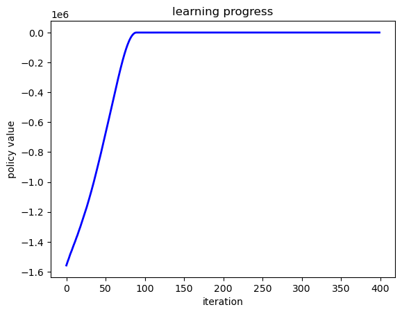
First we plot the evolution of lifetime value over the epochs.
# Plot learning progress
fig, ax = plt.subplots()
ax.plot(value_history, 'b-', linewidth=2)
ax.set_xlabel('iteration')
ax.set_ylabel('policy value')
ax.set_title('learning progress')
plt.show()
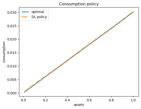
Next we compare the learned and optimal policies.
a_grid = jnp.linspace(0.01, 1.0, 1000)
policy_vmap = jax.vmap(lambda a: forward(params, a))
consumption_rate = policy_vmap(a_grid)
# Compute actual consumption: c = (c/a) * a
c_learned = consumption_rate * a_grid
c_optimal = κ * a_grid

fig, ax = plt.subplots()
ax.plot(a_grid, c_optimal, lw=2, label='optimal')
ax.plot(a_grid, c_learned, linestyle='--', lw=4, alpha=0.6, label='DL policy')
ax.set_xlabel('assets')
ax.set_ylabel('consumption')
ax.set_title('Consumption policy')
ax.legend()
plt.show()
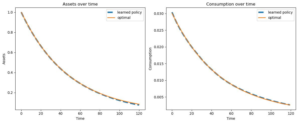
24.4.3. Simulation#
Let’s have a look at paths for consumption and assets under the learned and optimal policies.
The figures below show that the learned policies are close to optimal.
def simulate_consumption_path(
        params,   # ANN-based policy identified by params
        a_0,      # Initial condition
        T=120     # Simulation length
    ):
    # Simulate consumption and asset paths using ANN
    a = a_0
    a_sim, c_sim = [a], []
    for t in range(T):
        # Update policy path
        c = forward(params, a) * a
        c_sim.append(float(c))
        a = R * (a - c)
        a_sim.append(float(a))
        if a <= 1e-10:
            break

    # Simulate consumption and asset paths using optimal policy
    a = a_0
    a_opt, c_opt = [a], []
    for t in range(T):
        # Update optimal path
        c = κ * a
        c_opt.append(c)
        a = R * (a - c)
        a_opt.append(a)
        if a <= 1e-10:
            break

    return a_sim, c_sim, a_opt, c_opt
Let’s simulate and plot path
a_sim, c_sim, a_opt, c_opt = simulate_consumption_path(params, a_0=1.0)

fig, (ax1, ax2) = plt.subplots(1, 2, figsize=(12, 5))

ax1.plot(a_sim, lw=4, linestyle='--', label='learned policy')
ax1.plot(a_opt, lw=2, label='optimal')
ax1.set_xlabel('Time')
ax1.set_ylabel('Assets')
ax1.set_title('Assets over time')
ax1.legend()

ax2.plot(c_sim, lw=4, linestyle='--', label='learned policy')
ax2.plot(c_opt, lw=2, label='optimal')
ax2.set_xlabel('Time')
ax2.set_ylabel('Consumption')
ax2.set_title('Consumption over time')
ax2.legend()

plt.tight_layout()
plt.show()
24.5. IFP Model#
Now let’s solve a model with IID stochastic labor income using deep learning.
The set up was described at the start of this lecture.
24.5.1. JAX Implementation#
We start with a class called IFP that stores the model primitives.
class IFP(NamedTuple):
    R: float                 # Gross interest rate R = 1 + r
    β: float                 # Discount factor
    γ: float                 # Preference parameter
    z_mean: float            # Mean of log income shock
    z_std: float             # Std dev of log income shock
    z_samples: jnp.ndarray   # Std dev of log income shock


def create_ifp(
        r=0.01,
        β=0.96,
        γ=1.5,
        z_mean=0.1,
        z_std=0.1,
        n_shocks=200,
        seed=42
    ):
    R = 1 + r
    assert R * β < 1, "Stability condition violated."
    key = random.key(seed)
    z_samples = z_mean + z_std * jax.random.normal(key, n_shocks)
    return IFP(R, β, γ, z_mean, z_std, z_samples)
24.5.2. Solving the IID model using the EGM#
Since the shocks are IID, the optimal policy depends only on current assets \(a\).
For the IID normal case, we need to compute the expectation:
where \(Z \sim N(m, v)\) and \(Y = \exp(Z)\).
We approximate this expectation using Monte Carlo.
Here is the EGM operator \(K\) for the IID case:
def K(
        c_in: jnp.ndarray,       # Current consumption policy on endogenous grid
        a_in: jnp.ndarray,       # Current endogenous asset grid
        ifp: IFP,                # IFP model instance
        s_grid: jnp.ndarray,     # Exogenous savings grid
        n_shocks: int = 50       # Number of points for Monte Carlo integration
    ):
    """
    The Euler equation operator for the IFP model with IID shocks using EGM.

    """
    R, β, γ, z_mean, z_std, z_samples = ifp
    y_samples = jnp.exp(z_samples)
    u_prime = lambda c: c**(-γ)
    u_prime_inv = lambda c: c**(-1/γ)

    def compute_c_i(s_i):
        """Compute consumption for savings level s_i."""

        # For each income realization, compute next period assets and consumption
        def compute_mu_k(y_k):
            next_a = R * s_i + y_k
            # Interpolate to get consumption
            next_c = jnp.interp(next_a, a_in, c_in)
            return u_prime(next_c)

        # Compute expectation over income shocks (Monte Carlo average)
        mu_values = jax.vmap(compute_mu_k)(y_samples)
        expectation = jnp.mean(mu_values)

        # Invert to get consumption (handles s_i=0 case via smooth function)
        c = u_prime_inv(β * R * expectation)

        # For s_i = 0, consumption should be 0
        return jnp.where(s_i == 0, 0.0, c)

    # Compute consumption for all savings levels
    c_out = jax.vmap(compute_c_i)(s_grid)
    # Compute endogenous asset grid
    a_out = c_out + s_grid

    return c_out, a_out
Here’s the solver using time iteration:
def solve_model(
        ifp: IFP,                # IFP model instance
        s_grid: jnp.ndarray,     # Exogenous savings grid
        n_shocks: int = 50,      # Number of income shock realizations
        tol: float = 1e-5,       # Convergence tolerance
        max_iter: int = 1000     # Maximum iterations
    ):
    """
    Solve the IID model using time iteration with EGM.

    """
    # Initialize with consumption = assets (consume everything)
    a_init = s_grid.copy()
    c_init = s_grid.copy()
    c_in, a_in = c_init, a_init

    for i in range(max_iter):
        c_out, a_out = K(c_in, a_in, ifp, s_grid, n_shocks)

        error = jnp.max(jnp.abs(c_out - c_in))

        if error < tol:
            print(f"Converged in {i} iterations, error = {error:.2e}")
            break

        c_in, a_in = c_out, a_out

        if i % 100 == 0:
            print(f"Iteration {i}, error = {error:.2e}")

    return c_out, a_out
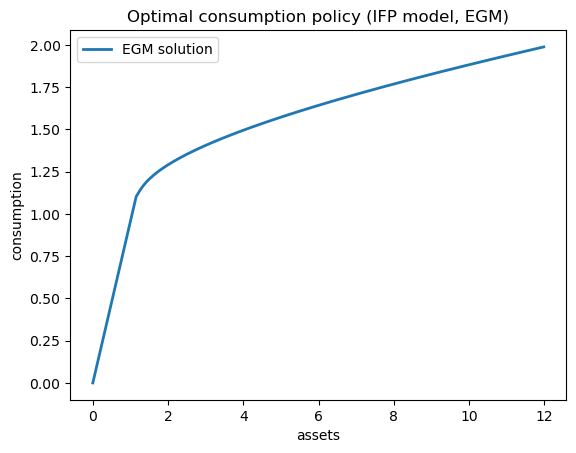
Let’s solve the model and plot the optimal policy:
# Create model instance
ifp = create_ifp(z_mean=0.1, z_std=0.1)

# Create savings grid
s_grid = jnp.linspace(0, 10, 200)

# Solve using EGM
print("Solving IFP model using EGM...\n")
c_egm, a_egm = solve_model(ifp, s_grid, n_shocks=100)
Solving IFP model using EGM...
Iteration 0, error = 1.40e+00
Converged in 38 iterations, error = 6.79e-06
Plot the optimal consumption policy:
fig, ax = plt.subplots()
ax.plot(a_egm, c_egm, lw=2, label='EGM solution')
ax.set_xlabel('assets')
ax.set_ylabel('consumption')
ax.set_title('Optimal consumption policy (IFP model, EGM)')
ax.legend()
plt.show()
24.5.3. Solving the IID model with DL#
Since the shocks are IID, the policy depends only on current assets \(a\).
We use the same network architecture as the deterministic case.
The forward pass uses the forward function from the deterministic case.
Here we implement lifetime value computation.
The key is to simulate paths with IID normal income shocks.
@partial(jax.jit, static_argnames=('path_length', 'num_paths'))
def compute_lifetime_value_ifp(
        params: list,            # Neural network parameters
        ifp: IFP,                # IFP model instance
        path_length: int,        # Length of each simulated path
        num_paths: int,          # Number of paths to simulate for averaging
        key: jax.Array           # JAX random key for generating income shocks
    ):
    """
    Compute expected lifetime value by averaging over multiple
    simulated paths.

    """
    R, β, γ, z_mean, z_std, z_samples = ifp

    def simulate_path(subkey):
        """Simulate a single path and return its lifetime value."""
        z_shocks = z_mean + z_std * jax.random.normal(subkey, path_length)
        Y = jnp.exp(z_shocks)

        def update(t, loop_state):
            a, value, discount = loop_state
            consumption_rate = forward(params, a)
            c = consumption_rate * a
            next_value = value + discount * u(c, γ)
            next_a = R * (a - c) + Y[t]
            next_discount = discount * β
            return next_a, next_value, next_discount

        initial_a = 10.0
        initial_value = 0.0
        initial_discount = 1.0
        initial_state = (initial_a, initial_value, initial_discount)
        final_a, final_value, final_discount = jax.lax.fori_loop(
            0, path_length, update, initial_state
        )

        return final_value

    # Generate keys for all paths
    path_keys = jax.random.split(key, num_paths)

    # Simulate all paths and average
    values = jax.vmap(simulate_path)(path_keys)
    return jnp.mean(values)
The loss function is the negation of the expected lifetime value.
def loss_function_ifp(params, ifp, path_length, num_paths, key):
    return -compute_lifetime_value_ifp(
        params, ifp, path_length, num_paths, key
    )
Now let’s set up and train the network.
We use the same ifp instance that was created for the EGM solution above.
config = Config()
key = random.key(config.seed)

print("Training IFP model with deep learning...\n")

# Set up loss function to pass to train_network
ifp_loss_fn = lambda params: loss_function_ifp(
    params, ifp, config.path_length, config.num_paths, key
)

# Warmup to trigger JIT compilation
print("Warming up JIT compilation...")
_ = train_network(config, ifp_loss_fn)

start_time = time.time()
ifp_params, ifp_value_history, best_ifp_value = train_network(
    config, ifp_loss_fn
)
best_ifp_value.block_until_ready()
elapsed = time.time() - start_time

print(f"\nBest value: {best_ifp_value:.4f}")
print(f"Final value: {ifp_value_history[-1]:.4f}")
print(f"Training time: {elapsed:.2f} seconds")
Training IFP model with deep learning...

Warming up JIT compilation...

Best value: -42.9578
Final value: -42.9578
Training time: 6.16 seconds
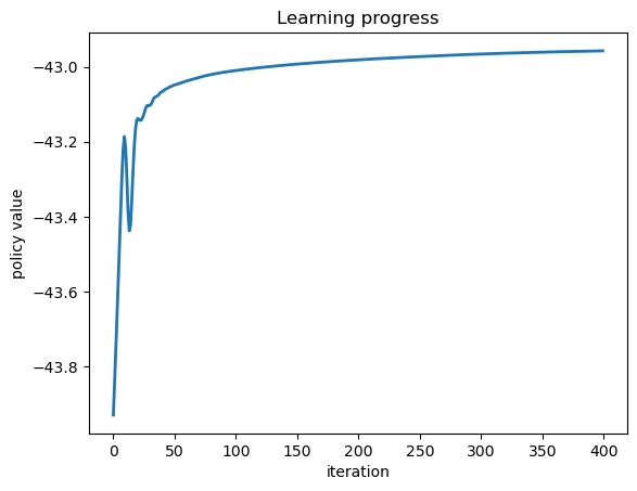
Plot the learning progress.
fig, ax = plt.subplots()
ax.plot(ifp_value_history, linewidth=2)
ax.set_xlabel('iteration')
ax.set_ylabel('policy value')
ax.set_title('Learning progress')
plt.show()
Compare EGM and DL solutions.
# Evaluate DL policy on asset grid
a_grid_dl = jnp.linspace(0.01, 10.0, 200)
policy_vmap = jax.vmap(lambda a: forward(ifp_params, a))
consumption_rate_dl = policy_vmap(a_grid_dl)
c_dl = consumption_rate_dl * a_grid_dl

fig, ax = plt.subplots()
ax.plot(a_egm, c_egm, lw=2, label='EGM solution')
ax.plot(a_grid_dl, c_dl, linestyle='--', lw=4, alpha=0.6, label='DL solution')
ax.set_xlabel('assets', fontsize=12)
ax.set_ylabel('consumption', fontsize=12)
ax.set_xlim(0, min(a_grid_dl[-1], a_egm[-1]))
ax.legend()
plt.show()
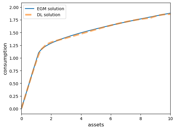
The fit is quite good.