4. Newton’s Method via JAX#
GPU
This lecture was built using a machine with access to a GPU — although it will also run without one.
Google Colab has a free tier with GPUs that you can access as follows:
Click on the “play” icon top right
Select Colab
Set the runtime environment to include a GPU
4.1. Overview#
One of the key features of JAX is automatic differentiation.
We introduced this feature in Adventures with Autodiff.
In this lecture we apply automatic differentiation to the problem of computing economic equilibria via Newton’s method.
Newton’s method is a relatively simple root and fixed point solution algorithm, which we discussed in a more elementary QuantEcon lecture.
JAX is ideally suited to implementing Newton’s method efficiently, even in high dimensions.
We use the following imports in this lecture
import jax
import jax.numpy as jnp
from scipy.optimize import root
import matplotlib.pyplot as plt
Let’s check the GPU we are running
!nvidia-smi
Thu Jul  9 05:42:36 2026
+-----------------------------------------------------------------------------------------+
| NVIDIA-SMI 580.105.08             Driver Version: 580.105.08     CUDA Version: 13.0     |
+-----------------------------------------+------------------------+----------------------+
| GPU  Name                 Persistence-M | Bus-Id          Disp.A | Volatile Uncorr. ECC |
| Fan  Temp   Perf          Pwr:Usage/Cap |           Memory-Usage | GPU-Util  Compute M. |
|                                         |                        |               MIG M. |
|=========================================+========================+======================|
|   0  Tesla T4                       On  |   00000000:00:1E.0 Off |                    0 |
| N/A   37C    P0             26W /   70W |       0MiB /  15360MiB |      0%      Default |
|                                         |                        |                  N/A |
+-----------------------------------------+------------------------+----------------------+

+-----------------------------------------------------------------------------------------+
| Processes:                                                                              |
|  GPU   GI   CI              PID   Type   Process name                        GPU Memory |
|        ID   ID                                                               Usage      |
|=========================================================================================|
|  No running processes found                                                             |
+-----------------------------------------------------------------------------------------+
4.2. Newton in one dimension#
As a warm up, let’s implement Newton’s method in JAX for a simple one-dimensional root-finding problem.
Let \(f\) be a function from \(\mathbb R\) to itself.
A root of \(f\) is an \(x \in \mathbb R\) such that \(f(x)=0\).
Recall that Newton’s method for solving for the root of \(f\) involves iterating with the map \(q\) defined by
Here is a function called newton that takes a function \(f\) plus a scalar value \(x_0\),
iterates with \(q\) starting from \(x_0\), and returns an approximate fixed point.
def newton(f, x_0, tol=1e-5):
    f_prime = jax.grad(f)
    def q(x):
        return x - f(x) / f_prime(x)

    error = tol + 1
    x = x_0
    while error > tol:
        y = q(x)
        error = abs(x - y)
        x = y

    return x
The code above uses automatic differentiation to calculate \(f'\) via the call to jax.grad.
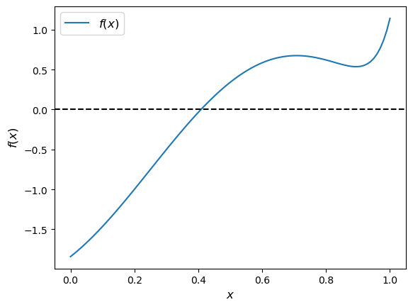
Let’s test our newton routine on the function shown below.
f = lambda x: jnp.sin(4 * (x - 1/4)) + x + x**20 - 1
x = jnp.linspace(0, 1, 100)

fig, ax = plt.subplots()
ax.plot(x, f(x), label='$f(x)$')
ax.axhline(ls='--', c='k')
ax.set_xlabel('$x$', fontsize=12)
ax.set_ylabel('$f(x)$', fontsize=12)
ax.legend(fontsize=12)
plt.show()
Here we go
newton(f, 0.2)
Array(0.4082935, dtype=float32, weak_type=True)
This number looks to be close to the root, given the figure.
4.3. An Equilibrium Problem#
Now let’s move up to higher dimensions.
First we describe a market equilibrium problem we will solve with JAX via root-finding.
The market is for \(n\) goods.
(We are extending a two-good version of the market from an earlier lecture.)
The supply function for the \(i\)-th good is
which we write in vector form as
(Here \(\sqrt{p}\) is the square root of each \(p_i\) and \(b \sqrt{p}\) is the vector formed by taking the pointwise product \(b_i \sqrt{p_i}\) at each \(i\).)
The demand function is
(Here \(A\) is an \(n \times n\) matrix containing parameters, \(c\) is an \(n \times 1\) vector and the \(\exp\) function acts pointwise (element-by-element) on the vector \(- A p\).)
The excess demand function is
An equilibrium price vector is an \(n\)-vector \(p\) such that \(e(p) = 0\).
The function below calculates the excess demand for given parameters
def e(p, A, b, c):
    return jnp.exp(- A @ p) + c - b * jnp.sqrt(p)
4.4. Computation#
In this section we describe and then implement the solution method.
4.4.1. Newton’s Method#
We use a multivariate version of Newton’s method to compute the equilibrium price.
The rule for updating a guess \(p_n\) of the equilibrium price vector is
Here \(J_e(p_n)\) is the Jacobian of \(e\) evaluated at \(p_n\).
Iteration starts from initial guess \(p_0\).
Instead of coding the Jacobian by hand, we use automatic differentiation via jax.jacobian().
def newton(f, x_0, tol=1e-5, max_iter=15):
    """
    A multivariate Newton root-finding routine.

    """
    x = x_0
    f_jac = jax.jacobian(f)
    @jax.jit
    def q(x):
        " Updates the current guess. "
        return x - jnp.linalg.solve(f_jac(x), f(x))
    error = tol + 1
    n = 0
    while error > tol:
        n += 1
        if(n > max_iter):
            raise Exception('Max iteration reached without convergence')
        y = q(x)
        error = jnp.linalg.norm(x - y)
        x = y
        print(f'iteration {n}, error = {error}')
    return x
4.4.2. Application#
Let’s now apply the method just described to investigate a large market with 5,000 goods.
We randomly generate the matrix \(A\) and set the parameter vectors \(b, c\) to \(1\).
dim = 5_000
seed = 32

# Create a random matrix A and normalize the rows to sum to one
key = jax.random.key(seed)
A = jax.random.uniform(key, [dim, dim])
s = jnp.sum(A, axis=0)
A = A / s

# Set up b and c
b = jnp.ones(dim)
c = jnp.ones(dim)
Here’s our initial condition \(p_0\)
init_p = jnp.ones(dim)
By combining the power of Newton’s method, JAX accelerated linear algebra, automatic differentiation, and a GPU, we obtain a relatively small error for this high-dimensional problem in just a few seconds:
%%time
p = newton(lambda p: e(p, A, b, c), init_p).block_until_ready()
iteration 1, error = 29.977436065673828
iteration 2, error = 5.092824935913086
iteration 3, error = 0.10971599072217941
iteration 4, error = 5.194256664253771e-05
iteration 5, error = 1.2965893802174833e-05
iteration 6, error = 6.7043965827906504e-06
CPU times: user 7.06 s, sys: 1.69 s, total: 8.76 s
Wall time: 9.19 s
We run it again to eliminate compile time.
%%time
p = newton(lambda p: e(p, A, b, c), init_p).block_until_ready()
iteration 1, error = 29.977436065673828
iteration 2, error = 5.092824935913086
iteration 3, error = 0.10971599072217941
iteration 4, error = 5.194256664253771e-05
iteration 5, error = 1.2965893802174833e-05
iteration 6, error = 6.7043965827906504e-06
CPU times: user 6.61 s, sys: 1.49 s, total: 8.1 s
Wall time: 8.7 s
Here’s the size of the error:
jnp.max(jnp.abs(e(p, A, b, c)))
Array(2.3841858e-07, dtype=float32)
With the same tolerance, SciPy’s root function takes much longer to run,
even with the Jacobian supplied.
%%time
solution = root(lambda p: e(p, A, b, c),
                init_p,
                jac=lambda p: jax.jacobian(e)(p, A, b, c),
                method='hybr',
                tol=1e-5)
CPU times: user 2min 31s, sys: 448 ms, total: 2min 31s
Wall time: 2min 31s
The result is also slightly less accurate:
p = solution.x
jnp.max(jnp.abs(e(p, A, b, c)))
Array(9.536743e-07, dtype=float32)
4.5. Exercises#
Exercise 4.1
Consider a three-dimensional extension of the Solow fixed point problem with
As before the law of motion is
However \(k_t\) is now a \(3 \times 1\) vector.
Solve for the fixed point using Newton’s method with the following initial values:
Hint
The computation of the fixed point is equivalent to computing \(k^*\) such that \(f(k^*) - k^* = 0\).
If you are unsure about your solution, you can start with the solved example:
with \(s = 0.3\), \(α = 0.3\), and \(δ = 0.4\) and starting value:
The result should converge to the analytical solution.
Solution
Let’s first define the parameters for this problem
A = jnp.array([[2.0, 3.0, 3.0],
               [2.0, 4.0, 2.0],
               [1.0, 5.0, 1.0]])
s = 0.2
α = 0.5
δ = 0.8
initLs = [jnp.ones(3),
          jnp.array([3.0, 5.0, 5.0]),
          jnp.repeat(50.0, 3)]
Then we define the multivariate version of the formula for the law of motion of capital
def multivariate_solow(k, A=A, s=s, α=α, δ=δ):
    return s * jnp.dot(A, k**α) + (1 - δ) * k
Let’s run through each starting value and see the output
attempt = 1
for init in initLs:
    print(f'Attempt {attempt}: Starting value is {init} \n')
    %time k = newton(lambda k: multivariate_solow(k) - k, \
                     init).block_until_ready()
    print('-'*64)
    attempt += 1
Attempt 1: Starting value is [1. 1. 1.]
iteration 1, error = 50.496315002441406
iteration 2, error = 41.1093864440918
iteration 3, error = 4.294127464294434
iteration 4, error = 0.3854290544986725
iteration 5, error = 0.0054382034577429295
iteration 6, error = 8.92080606718082e-07
CPU times: user 234 ms, sys: 16.1 ms, total: 250 ms
Wall time: 257 ms
----------------------------------------------------------------
Attempt 2: Starting value is [3. 5. 5.]

iteration 1, error = 2.0701100826263428
iteration 2, error = 0.12642373144626617
iteration 3, error = 0.0006017307168804109
iteration 4, error = 3.3717478231665154e-07
CPU times: user 154 ms, sys: 5.04 ms, total: 159 ms
Wall time: 121 ms
----------------------------------------------------------------
Attempt 3: Starting value is [50. 50. 50.]
iteration 1, error = 73.00942993164062
iteration 2, error = 6.493789196014404
iteration 3, error = 0.6806989312171936
iteration 4, error = 0.016202213242650032
iteration 5, error = 1.0600916539260652e-05
iteration 6, error = 9.830249609876773e-07
CPU times: user 338 ms, sys: 14.8 ms, total: 353 ms
Wall time: 294 ms
----------------------------------------------------------------
We find that the results are invariant to the starting values.
But the number of iterations it takes to converge is dependent on the starting values.
Let substitute the output back into the formulate to check our last result
multivariate_solow(k) - k
Array([ 4.7683716e-07, 0.0000000e+00, -2.3841858e-07], dtype=float32)
Note the error is very small.
We can also test our results on the known solution
A = jnp.array([[2.0, 0.0, 0.0],
               [0.0, 2.0, 0.0],
               [0.0, 0.0, 2.0]])
s = 0.3
α = 0.3
δ = 0.4
init = jnp.repeat(1.0, 3)
%time k = newton(lambda k: multivariate_solow(k, A=A, s=s, α=α, δ=δ) - k, \
                 init).block_until_ready()
iteration 1, error = 1.5745922327041626
iteration 2, error = 0.21344946324825287
iteration 3, error = 0.002045975998044014
iteration 4, error = 8.259061701210157e-07
CPU times: user 303 ms, sys: 17.2 ms, total: 320 ms
Wall time: 254 ms
# Now we time it without compile
%time k = newton(lambda k: multivariate_solow(k, A=A, s=s, α=α, δ=δ) - k, \
                 init).block_until_ready()
iteration 1, error = 1.5745922327041626
iteration 2, error = 0.21344946324825287
iteration 3, error = 0.002045975998044014
iteration 4, error = 8.259061701210157e-07
CPU times: user 305 ms, sys: 11.7 ms, total: 317 ms
Wall time: 240 ms
The result is very close to the true solution but still slightly different.
We can increase the precision of the floating point numbers and restrict the tolerance to obtain a more accurate approximation (see detailed discussion in the lecture on JAX)
# We will use 64 bit floats with JAX in order to increase the precision.
jax.config.update("jax_enable_x64", True)
init = init.astype('float64')

%time k = newton(lambda k: multivariate_solow(k, A=A, s=s, α=α, δ=δ) - k,\
                 init, tol=1e-7).block_until_ready()
iteration 1, error = 1.5745916432444333
iteration 2, error = 0.21344933091258958
iteration 3, error = 0.0020465547718452695
iteration 4, error = 2.0309190076799282e-07
iteration 5, error = 1.538370149106851e-15
CPU times: user 246 ms, sys: 11 ms, total: 257 ms
Wall time: 301 ms
# Now we time it without compile
%time k = newton(lambda k: multivariate_solow(k, A=A, s=s, α=α, δ=δ) - k,\
                 init, tol=1e-7).block_until_ready()
iteration 1, error = 1.5745916432444333
iteration 2, error = 0.21344933091258958
iteration 3, error = 0.0020465547718452695
iteration 4, error = 2.0309190076799282e-07
iteration 5, error = 1.538370149106851e-15
CPU times: user 136 ms, sys: 6.07 ms, total: 142 ms
Wall time: 125 ms
We can see it steps towards a more accurate solution.
Exercise 4.2
In this exercise, let’s try different initial values and check how Newton’s method responds to different starting points.
Let’s define a three-good problem with the following default values:
For this exercise, use the following extreme price vectors as initial values:
Set the tolerance to \(10^{-15}\) for more accurate output.
Hint
Similar to exercise 1, enabling float64 for JAX can improve the precision of our results.
Solution
Define parameters and initial values
A = jnp.array([
    [0.2, 0.1, 0.7],
    [0.3, 0.2, 0.5],
    [0.1, 0.8, 0.1]
])
b = jnp.array([1.0, 1.0, 1.0])
c = jnp.array([1.0, 1.0, 1.0])
initLs = [jnp.repeat(5.0, 3),
          jnp.array([4.5, 0.1, 4.0])]
Let’s run through each initial guess and check the output
attempt = 1
for init in initLs:
    print(f'Attempt {attempt}: Starting value is {init} \n')
    init = init.astype('float64')
    %time p = newton(lambda p: e(p, A, b, c), \
                 init, \
                 tol=1e-15, max_iter=15).block_until_ready()
    print('-'*64)
    attempt +=1
Attempt 1: Starting value is [5. 5. 5.]
iteration 1, error = 9.243805733085065
iteration 2, error = nan
CPU times: user 137 ms, sys: 4.21 ms, total: 141 ms
Wall time: 129 ms
----------------------------------------------------------------
Attempt 2: Starting value is [4.5 0.1 4. ]
iteration 1, error = 4.892018895185869
iteration 2, error = 1.2120550201694784
iteration 3, error = 0.6942087122866175
iteration 4, error = 0.168951089180319
iteration 5, error = 0.005209730313222213
iteration 6, error = 4.3632751705775364e-06
iteration 7, error = 3.0460818773540415e-12
iteration 8, error = 0.0
CPU times: user 130 ms, sys: 4.13 ms, total: 134 ms
Wall time: 116 ms
----------------------------------------------------------------
We can find that Newton’s method may fail for some starting values.
Sometimes it may take a few initial guesses to achieve convergence.
Substitute the result back to the formula to check our result
e(p, A, b, c)
Array([0., 0., 0.], dtype=float64)
We can see the result is very accurate.