10. Job Search#

GPU

This lecture was built using a machine with JAX installed and access to a GPU.

To run this lecture on Google Colab, click on the “play” icon top right, select Colab, and set the runtime environment to include a GPU.

To run this lecture on your own machine, you need to install Google JAX.

In this lecture we study a basic infinite-horizon job search problem with Markov wage draws

Note

For background on infinite horizon job search see, e.g., DP1.

The exercise at the end asks you to add risk-sensitive preferences and see how the main results change.

In addition to what’s in Anaconda, this lecture will need the following libraries:

!pip install quantecon

We use the following imports.

import matplotlib.pyplot as plt
import quantecon as qe
import jax
import jax.numpy as jnp
from collections import namedtuple

jax.config.update("jax_enable_x64", True)

10.1. Model#

We study an elementary model where

jobs are permanent
unemployed workers receive current compensation \(c\)
the horizon is infinite
an unemployment agent discounts the future via discount factor \(\beta \in (0,1)\)

10.1.1. Set up#

At the start of each period, an unemployed worker receives wage offer \(W_t\).

To build a wage offer process we consider the dynamics

\[ W_{t+1} = \rho W_t + \nu Z_{t+1} \]

where \((Z_t)_{t \geq 0}\) is IID and standard normal.

We then discretize this wage process using Tauchen’s method to produce a stochastic matrix \(P\).

Successive wage offers are drawn from \(P\).

10.1.2. Rewards#

Since jobs are permanent, the return to accepting wage offer \(w\) today is

\[ w + \beta w + \beta^2 w + \cdots = \frac{w}{1-\beta} \]

The Bellman equation is

\[ v(w) = \max \left\{ \frac{w}{1-\beta}, c + \beta \sum_{w'} v(w') P(w, w') \right\} \]

We solve this model using value function iteration.

10.2. Code#

Let’s set up a namedtuple to store information needed to solve the model.

Model = namedtuple('Model', ('n', 'w_vals', 'P', 'β', 'c'))

The function below holds default values and populates the namedtuple.

def create_js_model(
        n=500,       # wage grid size
        ρ=0.9,       # wage persistence
        ν=0.2,       # wage volatility
        β=0.99,      # discount factor
        c=1.0,       # unemployment compensation
    ):
    "Creates an instance of the job search model with Markov wages."
    mc = qe.tauchen(n, ρ, ν)
    w_vals, P = jnp.exp(mc.state_values), jnp.array(mc.P)
    return Model(n, w_vals, P, β, c)

Let’s test it:

model = create_js_model(β=0.98)

model.c

1.0

model.β

0.98

model.w_vals.mean()  

Array(1.34861482, dtype=float64)

Here’s the Bellman operator.

@jax.jit
def T(v, model):
    """
    The Bellman operator Tv = max{e, c + β E v} with 

        e(w) = w / (1-β) and (Ev)(w) = E_w[ v(W')]

    """
    n, w_vals, P, β, c = model
    h = c + β * P @ v
    e = w_vals / (1 - β)

    return jnp.maximum(e, h)

The next function computes the optimal policy under the assumption that \(v\) is the value function.

The policy takes the form

\[ \sigma(w) = \mathbf 1 \left\{ \frac{w}{1-\beta} \geq c + \beta \sum_{w'} v(w') P(w, w') \right\} \]

Here \(\mathbf 1\) is an indicator function.

\(\sigma(w) = 1\) means stop
\(\sigma(w) = 0\) means continue.

@jax.jit
def get_greedy(v, model):
    "Get a v-greedy policy."
    n, w_vals, P, β, c = model
    e = w_vals / (1 - β)
    h = c + β * P @ v
    σ = jnp.where(e >= h, 1, 0)
    return σ

Here’s a routine for value function iteration.

def vfi(model, max_iter=10_000, tol=1e-4):
    "Solve the infinite-horizon Markov job search model by VFI."
    print("Starting VFI iteration.")
    v = jnp.zeros_like(model.w_vals)    # Initial guess
    i = 0
    error = tol + 1

    while error > tol and i < max_iter:
        new_v = T(v, model)
        error = jnp.max(jnp.abs(new_v - v))
        i += 1
        v = new_v

    v_star = v
    σ_star = get_greedy(v_star, model)
    return v_star, σ_star

10.3. Computing the solution#

Let’s set up and solve the model.

model = create_js_model()
n, w_vals, P, β, c = model

v_star, σ_star = vfi(model)

Starting VFI iteration.

Here’s the optimal policy:

fig, ax = plt.subplots()
ax.plot(σ_star)
ax.set_xlabel("wage values")
ax.set_ylabel("optimal choice (stop=1)")
plt.show()

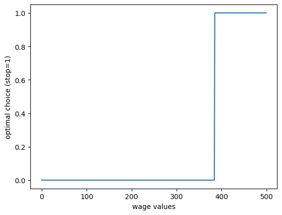
_images/37f92b538d37a0b6693cccc0cd2e7cd0db6a2f95f771c4b9c52d3216c2d2ec10.png

We compute the reservation wage as the first \(w\) such that \(\sigma(w)=1\).

stop_indices = jnp.where(σ_star == 1)
stop_indices

(Array([385, 386, 387, 388, 389, 390, 391, 392, 393, 394, 395, 396, 397,
        398, 399, 400, 401, 402, 403, 404, 405, 406, 407, 408, 409, 410,
        411, 412, 413, 414, 415, 416, 417, 418, 419, 420, 421, 422, 423,
        424, 425, 426, 427, 428, 429, 430, 431, 432, 433, 434, 435, 436,
        437, 438, 439, 440, 441, 442, 443, 444, 445, 446, 447, 448, 449,
        450, 451, 452, 453, 454, 455, 456, 457, 458, 459, 460, 461, 462,
        463, 464, 465, 466, 467, 468, 469, 470, 471, 472, 473, 474, 475,
        476, 477, 478, 479, 480, 481, 482, 483, 484, 485, 486, 487, 488,
        489, 490, 491, 492, 493, 494, 495, 496, 497, 498, 499],      dtype=int64),)

res_wage_index = min(stop_indices[0])

res_wage = w_vals[res_wage_index]

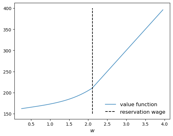
Here’s a joint plot of the value function and the reservation wage.

fig, ax = plt.subplots()
ax.plot(w_vals, v_star, alpha=0.8, label="value function")
ax.vlines((res_wage,), 150, 400, 'k', ls='--', label="reservation wage")
ax.legend(frameon=False, fontsize=12, loc="lower right")
ax.set_xlabel("$w$", fontsize=12)
plt.show()

_images/72b5dbe7759fc42dc33eb063f29db1473fd7b3a472279e651707faee1acb3239.png

10.4. Exercise#

Exercise 10.1

In the setting above, the agent is risk-neutral vis-a-vis future utility risk.

Now solve the same problem but this time assuming that the agent has risk-sensitive preferences, which are a type of nonlinear recursive preferences.

The Bellman equation becomes

\[ v(w) = \max \left\{ \frac{w}{1-\beta}, c + \frac{\beta}{\theta} \ln \left[ \sum_{w'} \exp(\theta v(w')) P(w, w') \right] \right\} \]

When \(\theta < 0\) the agent is risk averse.

Solve the model when \(\theta = -0.1\) and compare your result to the risk neutral case.

Try to interpret your result.

You can start with the following code:

RiskModel = namedtuple('Model', ('n', 'w_vals', 'P', 'β', 'c', 'θ'))

def create_risk_sensitive_js_model(
        n=500,       # wage grid size
        ρ=0.9,       # wage persistence
        ν=0.2,       # wage volatility
        β=0.99,      # discount factor
        c=1.0,       # unemployment compensation
        θ=-0.1       # risk parameter
    ):
    "Creates an instance of the job search model with Markov wages."
    mc = qe.tauchen(n, ρ, ν)
    w_vals, P = jnp.exp(mc.state_values), mc.P
    P = jnp.array(P)
    return RiskModel(n, w_vals, P, β, c, θ)

Now you need to modify T and get_greedy and then run value function iteration again.

Solution to Exercise 10.1

RiskModel = namedtuple('Model', ('n', 'w_vals', 'P', 'β', 'c', 'θ'))

def create_risk_sensitive_js_model(
        n=500,       # wage grid size
        ρ=0.9,       # wage persistence
        ν=0.2,       # wage volatility
        β=0.99,      # discount factor
        c=1.0,       # unemployment compensation
        θ=-0.1       # risk parameter
    ):
    "Creates an instance of the job search model with Markov wages."
    mc = qe.tauchen(n, ρ, ν)
    w_vals, P = jnp.exp(mc.state_values), mc.P
    P = jnp.array(P)
    return RiskModel(n, w_vals, P, β, c, θ)


@jax.jit
def T_rs(v, model):
    """
    The Bellman operator Tv = max{e, c + β R v} with 

        e(w) = w / (1-β) and

        (Rv)(w) = (1/θ) ln{E_w[ exp(θ v(W'))]}

    """
    n, w_vals, P, β, c, θ = model
    h = c + (β / θ) * jnp.log(P @ (jnp.exp(θ * v)))
    e = w_vals / (1 - β)

    return jnp.maximum(e, h)


@jax.jit
def get_greedy_rs(v, model):
    " Get a v-greedy policy."
    n, w_vals, P, β, c, θ = model
    e = w_vals / (1 - β)
    h = c + (β / θ) * jnp.log(P @ (jnp.exp(θ * v)))
    σ = jnp.where(e >= h, 1, 0)
    return σ



def vfi(model, max_iter=10_000, tol=1e-4):
    "Solve the infinite-horizon Markov job search model by VFI."
    print("Starting VFI iteration.")
    v = jnp.zeros_like(model.w_vals)    # Initial guess
    i = 0
    error = tol + 1

    while error > tol and i < max_iter:
        new_v = T_rs(v, model)
        error = jnp.max(jnp.abs(new_v - v))
        i += 1
        v = new_v

    v_star = v
    σ_star = get_greedy_rs(v_star, model)
    return v_star, σ_star



model_rs = create_risk_sensitive_js_model()

n, w_vals, P, β, c, θ = model_rs

v_star_rs, σ_star_rs = vfi(model_rs)

Starting VFI iteration.

Let’s plot the results together with the original risk neutral case and see what we get.

stop_indices = jnp.where(σ_star_rs == 1)
res_wage_index = min(stop_indices[0])
res_wage_rs = w_vals[res_wage_index]

fig, ax = plt.subplots()
ax.plot(w_vals, v_star,  alpha=0.8, label="risk neutral $v$")
ax.plot(w_vals, v_star_rs, alpha=0.8, label="risk sensitive $v$")
ax.vlines((res_wage,), 100, 400,  ls='--', color='darkblue', 
          alpha=0.5, label=r"risk neutral $\bar w$")
ax.vlines((res_wage_rs,), 100, 400, ls='--', color='orange', 
          alpha=0.5, label=r"risk sensitive $\bar w$")
ax.legend(frameon=False, fontsize=12, loc="lower right")
ax.set_xlabel("$w$", fontsize=12)
plt.show()

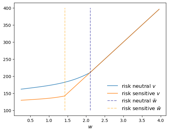
_images/e9783e98f9243d0eacfd26651a9967a32632a0196b5280c4c558de33b37e7622.png

The figure shows that the reservation wage under risk sensitive preferences (RS \(\bar w\)) shifts down.

This makes sense – the agent does not like risk and hence is more inclined to accept the current offer, even when it’s lower.