26. Schelling Model with NumPy

26.1. Overview

In the previous lecture, we implemented the Schelling segregation model using pure Python and standard libraries, rather than Python plus numerical and scientific libraries.

In this lecture, we rewrite the model using NumPy arrays and functions.

NumPy is the most fundamental library for numerical coding in Python.

We’ll achieve greater speed — but at the cost of readability!

import matplotlib.pyplot as plt
import numpy as np
from numpy.random import uniform
import time

26.2. Data Representation

In the class-based version, each agent was an object storing its own type and location.

Here we take a different approach: we store all agent data in NumPy arrays.

• locations — an \(n \times 2\) array where row \(i\) holds the \((x, y)\) coordinates of agent \(i\)

• types — an array of length \(n\) where entry \(i\) is 0 or 1, indicating agent \(i\)’s type

Let’s set up the parameters:

num_of_type_0 = 1000    # number of agents of type 0 (orange)
num_of_type_1 = 1000    # number of agents of type 1 (green)
n = num_of_type_0 + num_of_type_1  # total number of agents
num_neighbors = 10      # number of agents viewed as neighbors
max_other_type = 6      # max number of different-type neighbors tolerated

Here’s a function to initialize the state with random locations and types:

def initialize_state():
    locations = uniform(size=(n, 2))
    types = np.array([0] * num_of_type_0 + [1] * num_of_type_1)
    return locations, types

Let’s see what this looks like:

np.random.seed(1234)
locations, types = initialize_state()

print(f"locations shape: {locations.shape}")
print(f"First 5 locations:\n{locations[:5]}")
print(f"\ntypes shape: {types.shape}")
print(f"First 20 types: {types[:20]}")

locations shape: (2000, 2)
First 5 locations:
[[0.19151945 0.62210877]
 [0.43772774 0.78535858]
 [0.77997581 0.27259261]
 [0.27646426 0.80187218]
 [0.95813935 0.87593263]]

types shape: (2000,)
First 20 types: [0 0 0 0 0 0 0 0 0 0 0 0 0 0 0 0 0 0 0 0]

26.3. Helper Functions

Let’s write some functions that compute what we need while operating on the arrays.

26.3.1. Computing Distances

To find an agent’s neighbors, we need to compute distances.

def get_distances(loc, locations):
    """
    Compute the Euclidean distance from one location to all agent locations.

    """
    return np.linalg.norm(loc - locations, axis=1)

Let’s break down how this function works:

1. loc - locations subtracts the reference point loc from every row of locations. NumPy “broadcasts” the subtraction, so if loc = [0.5, 0.3] and locations has 2000 rows, the result is a 2000 × 2 array where each row is the difference vector from loc to that agent.

2. np.linalg.norm(..., axis=1) computes the Euclidean norm of each row. The axis=1 argument tells NumPy to compute the norm across columns (i.e., for each row separately).

This vectorized approach is much faster than looping through agents one by one.

26.3.2. Finding Neighbors

Now we can find the nearest neighbors:

def get_neighbors(i, locations):
    " Get indices of the nearest neighbors to agent i (excluding self). "
    loc = locations[i, :]
    distances = get_distances(loc, locations)
    distances[i] = np.inf                 # Don't count ourselves 
    indices = np.argsort(distances)       # Sort agents by distance
    neighbors = indices[:num_neighbors]   # Keep the closest
    return neighbors

Here’s how this function works:

1. First we call get_distances to get an array of 2000 distances (one for each agent).

2. We set distances[i] = np.inf so that agent \(i\) doesn’t count as their own neighbor.

3. np.argsort(distances) returns the indices of agents sorted from closest to furthest. For example, if the closest agent has index 42, then indices[0] equals 42.

4. indices[:num_neighbors] uses slicing to keep only the first num_neighbors indices — these correspond to the nearest neighbors.

# Find neighbors of agent 0
neighbors = get_neighbors(0, locations)
print(f"Agent 0's nearest neighbors: {neighbors}")
print(f"Agent 0 is NOT included: {0 not in neighbors}")

Agent 0's nearest neighbors: [ 595 1737  366 1442 1283  261  763  854 1427  218]
Agent 0 is NOT included: True

26.3.3. Checking Happiness

An agent is happy if enough of their neighbors share their type:

def is_happy(i, locations, types):
    " True if agent i has no more than max_other_type neighbors of a different type. "
    agent_type = types[i]
    neighbors = get_neighbors(i, locations)
    neighbor_types = types[neighbors]
    num_other = np.sum(neighbor_types != agent_type)
    return num_other <= max_other_type

Let’s walk through this function step by step:

1. types[i] gets the type (0 or 1) of agent \(i\).

2. get_neighbors(i, locations) returns an array of indices for the nearest neighbors.

3. types[neighbors] uses these indices to look up the types of the neighbors. This is called “fancy indexing” — when you pass an array of indices to another array, NumPy returns the elements at those positions. For example, if neighbors = [42, 7, 15, ...], then types[neighbors] returns [types[42], types[7], types[15], ...].

4. neighbor_types == agent_type compares each neighbor’s type to the agent’s type, producing an array of True/False values (e.g., [True, False, True, ...]).

5. np.sum(...) counts how many True values there are. In NumPy, True is treated as 1 and False as 0, so summing a boolean array counts the True entries.

6. Finally, we check if this count is within the tolerance max_other_type.

# Check if agent 0 is happy
print(f"Agent 0 type: {types[0]}")
print(f"Agent 0 happy: {is_happy(0, locations, types)}")

Agent 0 type: 0
Agent 0 happy: True

26.3.4. Counting Happy Agents

The next function uses a loop to check each agent and count how many are happy.

def count_happy(locations, types):
    " Count the number of happy agents. "
    happy_count = 0
    for i in range(n):
        happy_count += is_happy(i, locations, types)
    return happy_count

Since is_happy returns True or False, and Python treats True as 1 when adding, we can accumulate the count directly.

print(f"Initially happy agents: {count_happy(locations, types)} out of {n}")

Initially happy agents: 1648 out of 2000

26.3.5. Moving Unhappy Agents

When an agent is unhappy, they keep trying new random locations until they find one where they’re happy:

def update_agent(i, locations, types, max_attempts=10_000):
    " Move agent i to a new location where they are happy. "
    attempts = 0
    while not is_happy(i, locations, types):
        locations[i, :] = uniform(), uniform()
        attempts += 1
        if attempts >= max_attempts:
            break

Here’s how this works:

1. The while loop keeps running as long as the agent is unhappy.

2. locations[i, :] = uniform(), uniform() assigns a new random \((x, y)\) location to agent \(i\). The left side locations[i, :] selects row \(i\) (all columns), and the right side creates a tuple of two random numbers between 0 and 1.

3. Importantly, this modifies the locations array in place. We don’t need to return anything because the original array is changed directly. This is a key feature of NumPy arrays — when you modify a slice, you modify the underlying data.

26.4. Visualization

Here’s some code for Visualization — we’ll skip the details

def plot_distribution(locations, types, title):
    " Plot the distribution of agents. "
    fig, ax = plt.subplots()
    plot_args = {
        'markersize': 6, 'alpha': 0.8, 
        'markeredgecolor': 'black', 
        'markeredgewidth': 0.5
    }
    colors = 'darkorange', 'green'
    for agent_type, color in zip((0, 1), colors):
        idx = (types == agent_type)
        ax.plot(locations[idx, 0],
                locations[idx, 1],
                'o',
                markerfacecolor=color,
                **plot_args)
    ax.set_title(title)
    plt.show()

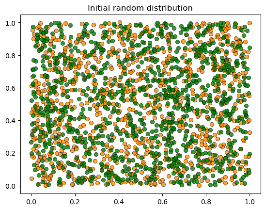
Let’s visualize the initial random distribution:

np.random.seed(1234)
locations, types = initialize_state()
plot_distribution(locations, types, 'Initial random distribution')

26.5. The Simulation

Now we put it all together.

As in the first lecture, each iteration cycles through all agents in order, giving each the opportunity to move:

def run_simulation(max_iter=100_000, seed=42):
    """
    Run the Schelling simulation.

    Each iteration cycles through all agents, giving each a chance to move.
    """
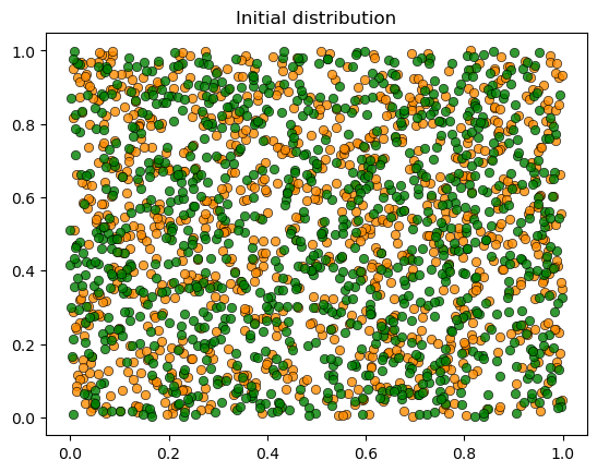
    np.random.seed(seed)
    locations, types = initialize_state()

    plot_distribution(locations, types, 'Initial distribution')

    # Loop until no agent wishes to move
    start_time = time.time()
    someone_moved = True
    iteration = 0
    while someone_moved and iteration < max_iter:
        print(f'Entering iteration {iteration + 1}')
        iteration += 1
        someone_moved = False
        for i in range(n):
            if not is_happy(i, locations, types):
                update_agent(i, locations, types)
                someone_moved = True
    elapsed = time.time() - start_time

    plot_distribution(locations, types, f'Iteration {iteration}')

    if not someone_moved:
        print(f'Converged in {elapsed:.2f} seconds after {iteration} iterations.')
    else:
        print('Hit iteration bound and terminated.')

    return locations, types

26.6. Results

Let’s run the simulation:

locations, types = run_simulation()

Entering iteration 1
Entering iteration 2
Entering iteration 3
Entering iteration 4
Entering iteration 5
Entering iteration 6
Entering iteration 7
Converged in 1.86 seconds after 7 iterations.

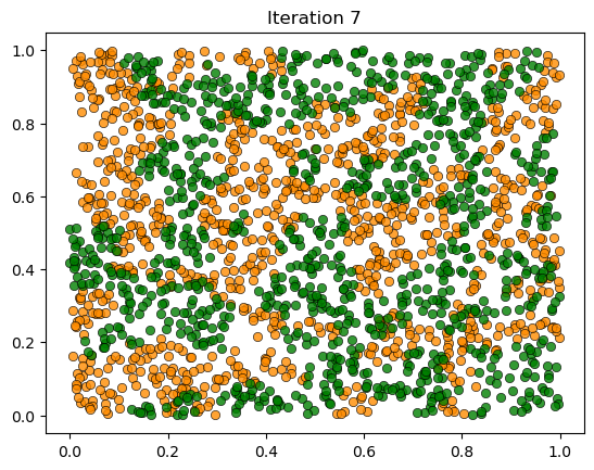
We see the same phenomenon as in the class-based version: starting from a random mixed distribution, agents self-organize into segregated clusters.