29. Segregation with Persistent Shocks#
29.1. Overview#
In previous lectures, we saw that the Schelling model converges to a segregated equilibrium: agents relocate until everyone is happy, and then the system stops.
But real cities don’t work this way. People move in and out, neighborhoods change, and the population is constantly being reshuffled by small shocks.
In this lecture, we explore what happens when we add this kind of persistent randomness to the model.
Specifically, after each iteration, we randomly flip the type of some agents with a small probability.
We can interpret this as agents occasionally moving away and being replaced by new agents whose type is randomly determined.
With persistent shocks, the system never converges, so the segregation dynamics keep operating indefinitely.
Because agents are constantly being nudged out of equilibrium, the forces that drive segregation never shut off.
The result is that segregation levels continue to increase over time, reaching levels beyond what we see in the basic model.
We use the parallel JAX implementation for efficiency, allowing us to run longer simulations with more agents.
import matplotlib.pyplot as plt
import numpy as np
import jax
import jax.numpy as jnp
from jax import random, jit, vmap
from functools import partial
from typing import NamedTuple
import time
29.2. Parameters#
We use 2000 agents of each type and add a flip_prob parameter that controls
the probability of an agent’s type being flipped after each iteration.
class Params(NamedTuple):
    num_of_type_0: int = 2000    # number of agents of type 0 (orange)
    num_of_type_1: int = 2000    # number of agents of type 1 (green)
    num_neighbors: int = 10      # number of neighbors
    max_other_type: int = 6      # max number of different-type neighbors tolerated
    num_candidates: int = 3      # candidate locations per agent per iteration
    flip_prob: float = 0.01      # probability of flipping an agent's type


params = Params()
29.3. Setup#
The following functions are repeated from the previous lecture:
29.4. Type Flipping#
This is the key addition in this lecture. After each iteration, we randomly
flip the type of each agent with probability flip_prob.
@partial(jit, static_argnames=('params',))
def flip_types(types, key, params):
    """
    Randomly flip agent types with probability flip_prob.
    """
    n = params.num_of_type_0 + params.num_of_type_1
    flip_prob = params.flip_prob

    # Generate random numbers for each agent
    random_vals = random.uniform(key, n)

    # Determine which agents get flipped
    should_flip = random_vals < flip_prob

    # Flip: 0 -> 1, 1 -> 0  (equivalent to 1 - type)
    flipped_types = 1 - types

    # Apply flips only where should_flip is True
    new_types = jnp.where(should_flip, flipped_types, types)

    return new_types
29.5. Simulation with Shocks#
The simulation loop now includes type flipping after each iteration. We run for a fixed number of iterations rather than waiting for convergence, since the system will never fully converge with ongoing shocks.
def run_simulation_with_shocks(params, max_iter=1000, seed=42, plot_every=100):
"""
Run the Schelling simulation with random type flips.
Parameters
----------
params : Params
Model parameters including flip_prob.
max_iter : int
Number of iterations to run.
seed : int
Random seed.
plot_every : int
Plot the distribution every this many iterations.
"""
key = random.key(seed)
key, init_key = random.split(key)
locations, types = initialize_state(init_key, params)
n = locations.shape[0]
print(f"Running simulation with {n} agents for {max_iter} iterations")
print(f"Flip probability: {params.flip_prob}")
print()
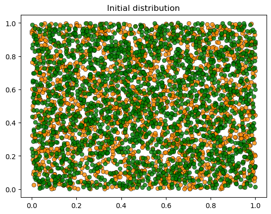
plot_distribution(locations, types, 'Initial distribution')
start_time = time.time()
for iteration in range(1, max_iter + 1):
# Update locations (agents try to find happy spots)
locations, key = parallel_update_step(locations, types, key, params)
# Apply random type flips
key, flip_key = random.split(key)
types = flip_types(types, flip_key, params)
# Periodically report progress and plot
if iteration % plot_every == 0:
unhappy = get_unhappy_agents(locations, types, params)
elapsed = time.time() - start_time
print(f'Iteration {iteration}: {int(jnp.sum(unhappy))} unhappy agents, {elapsed:.1f}s elapsed')
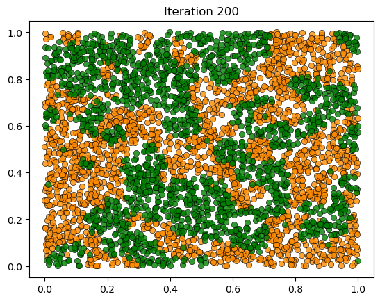
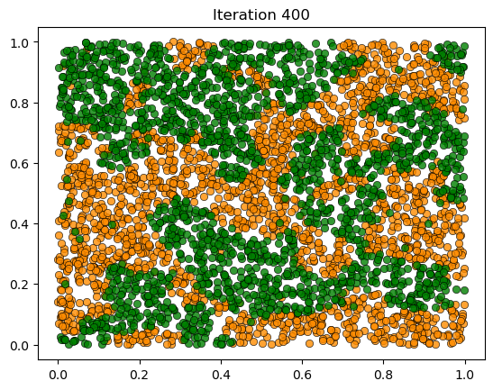
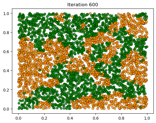
plot_distribution(locations, types, f'Iteration {iteration}')
elapsed = time.time() - start_time
print(f'\nCompleted {max_iter} iterations in {elapsed:.2f} seconds.')
return locations, types
29.6. Results#
Let’s warm up the JIT-compiled functions and run the simulation:
key = random.key(0)
key, init_key = random.split(key)
test_locations, test_types = initialize_state(init_key, params)

_ = is_happy(test_locations[0], 0, test_locations, test_types, params)
_ = get_unhappy_agents(test_locations, test_types, params)
key, subkey = random.split(key)
_ = update_agent_location(0, test_locations, test_types, subkey, params)
key, subkey = random.split(key)
_, _ = parallel_update_step(test_locations, test_types, subkey, params)
key, subkey = random.split(key)
_ = flip_types(test_types, subkey, params)

print("JAX functions compiled and ready!")
JAX functions compiled and ready!
locations, types = run_simulation_with_shocks(params, max_iter=1000, plot_every=200)
Running simulation with 4000 agents for 1000 iterations
Flip probability: 0.01
Iteration 200: 48 unhappy agents, 3.3s elapsed
Iteration 400: 57 unhappy agents, 6.8s elapsed
Iteration 600: 57 unhappy agents, 10.2s elapsed
Iteration 800: 48 unhappy agents, 13.6s elapsed
Iteration 1000: 45 unhappy agents, 17.1s elapsed

Completed 1000 iterations in 17.36 seconds.
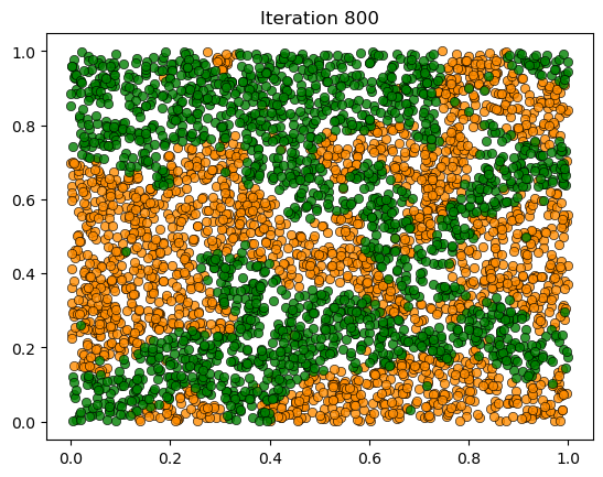
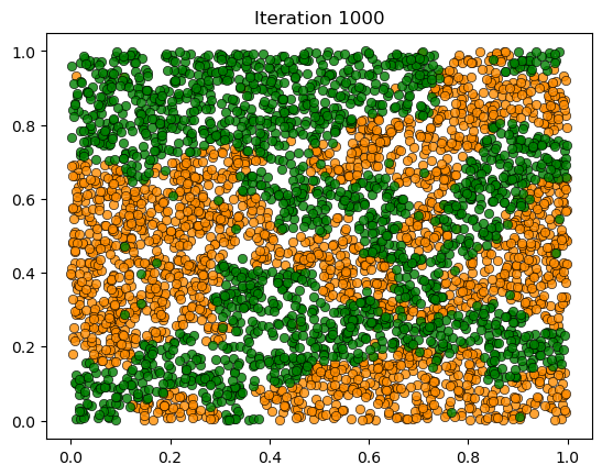
29.7. Discussion#
The figures show an interesting result: segregation levels at the end of the simulation are much higher than in the basic model without shocks.
Why does this happen?
In the basic model, the system converges to an equilibrium where everyone is happy, and then the dynamics stop.
With persistent shocks, the system never converges — random type flips create local pockets of unhappiness, triggering relocations that can cascade through the population.
The key insight is that the segregation dynamics never shut off.
The result is that segregation continues to increase over time, reaching levels far beyond what we observe when the system is allowed to converge.
This is arguably more realistic than the static equilibrium of the basic model.
Real cities experience constant population turnover, and the Schelling dynamics operate continuously on the evolving population.